class: center, middle, inverse # Power Analysis and Null Hypothesis Testing  --- # We've Talked About P-Values and Null Hypothesis Testing as a Means of Inference - For Industrial Quality Control, NHST was introduced to establish cutoffs of reasonable p, called an `\(\alpha\)` - This corresponds to Confidence intervals: 1 - `\(\alpha\)` = CI of interest - Results with p `\(\le\)` `\(\alpha\)` are deemed **statistically significant** --- # Alpha is Important as It Prevents us From Making Misguided Statements 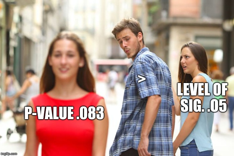 --- # Although if P is Continuous, You Avoid This - Mostly 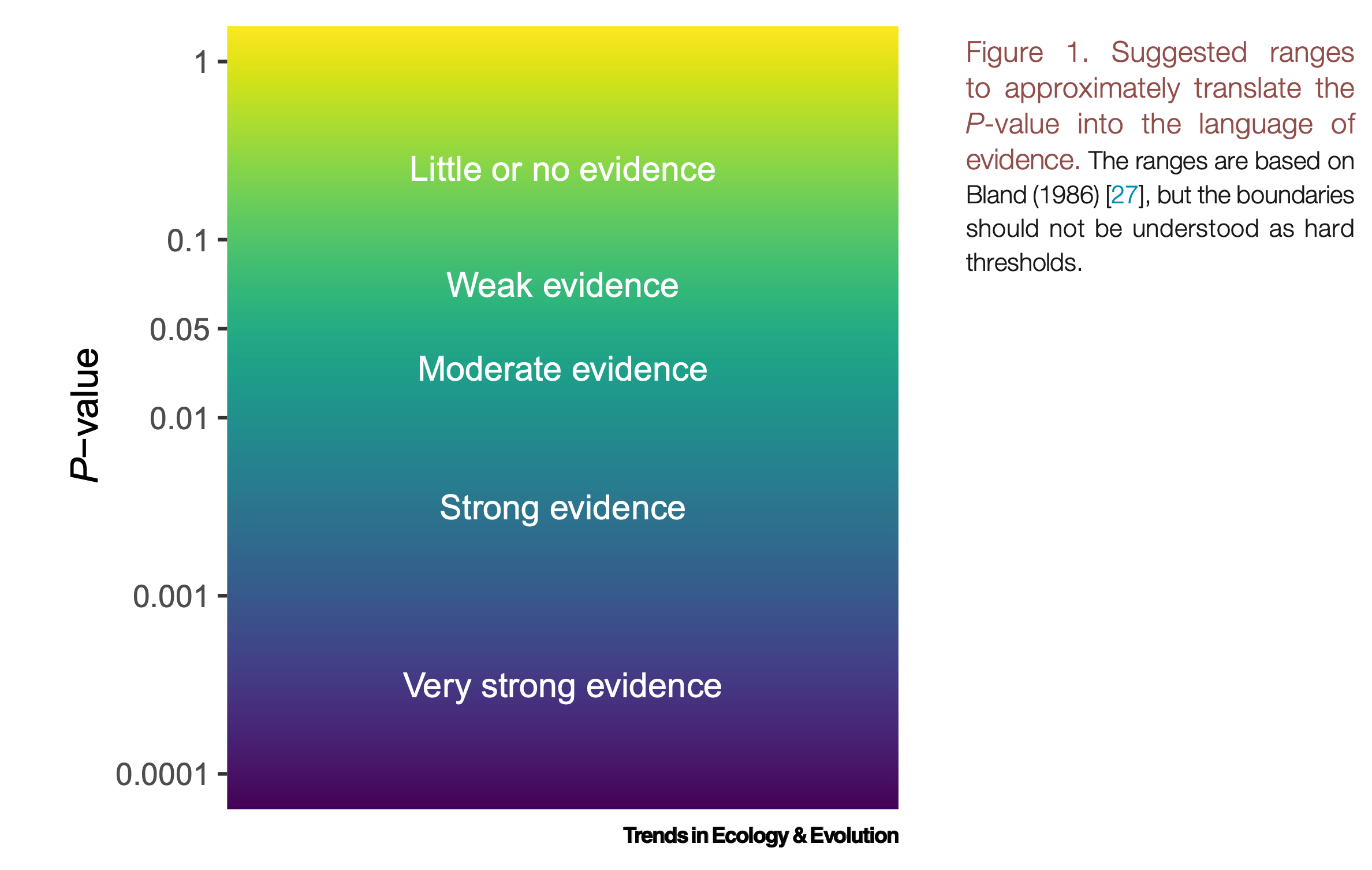 Muff et al. 2022 TREE --- class:middle # Even So, You Can Still Make Mistakes .pull-left[] -- .pull-right[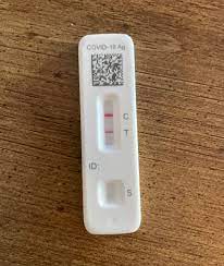 ] -- .bottom[ You reject that null that everything is OK - but you're wrong! False Positive! AKA **TYPE I ERROR**] --- class:center, middle # `\(\Large \alpha\)` is the probability of comitting a Type I error - getting a False Positive --- # You Could Also Have a False Negative! .pull-left[] -- .pull-right[] -- .bottom[ .center[You fail to reject your null incorrectly - **Type II Error**] ] --- class:center, middle # `\(\Large \beta\)` is the probability of comitting a Type II error - getting a False Negative --- # Null Hypothesis: This is Not a Hotdog .center[ .middle[ 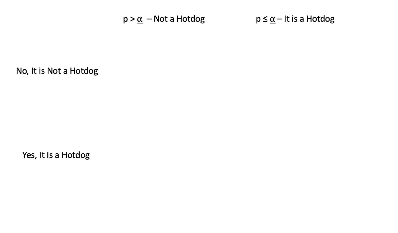 ] ] --- # Null Hypothesis: This is Not a Hotdog .center[ .middle[ 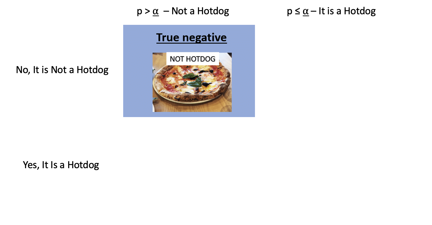 ] ] --- # Null Hypothesis: This is Not a Hotdog .center[ .middle[ 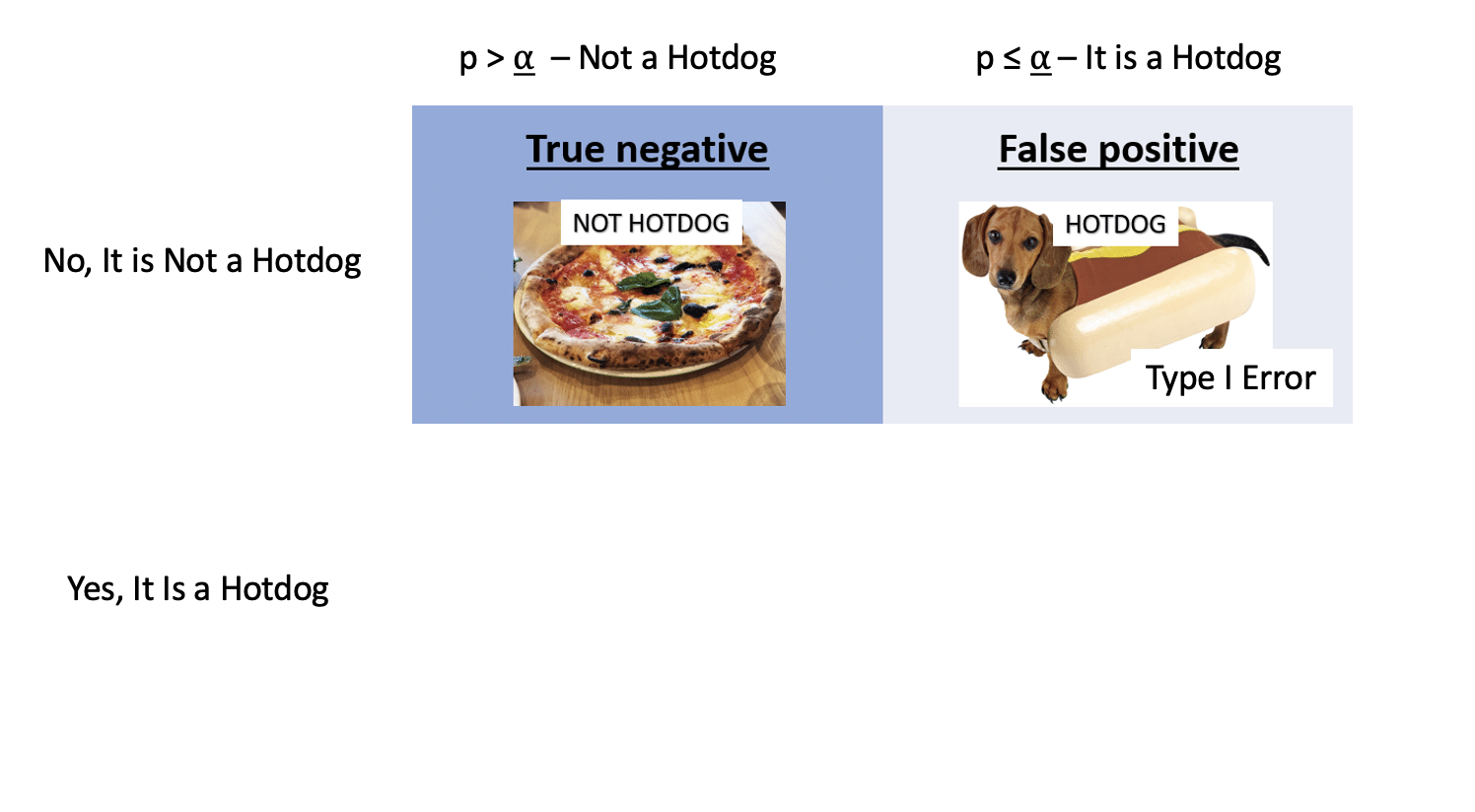 ] ] --- # Null Hypothesis: This is Not a Hotdog .center[ .middle[ 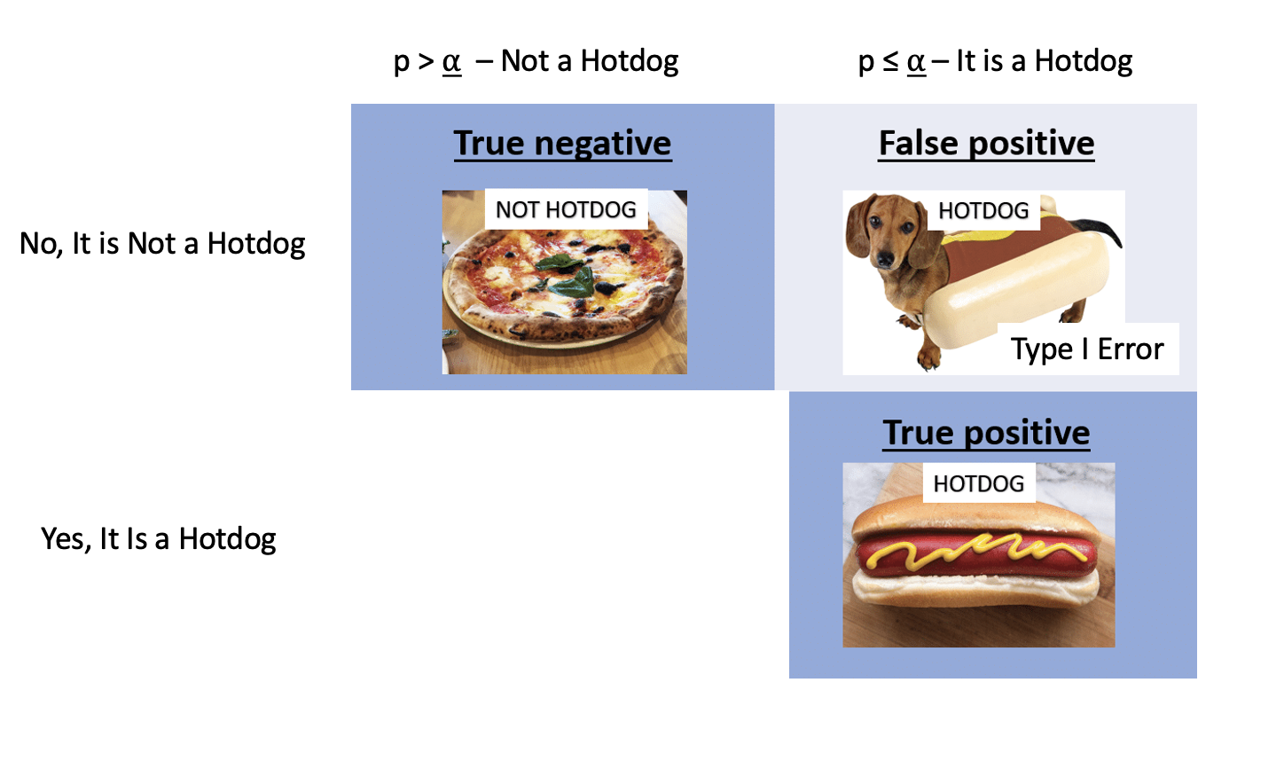 ] ] --- # Null Hypothesis: This is Not a Hotdog .center[ .middle[  ] ] --- # Types of Errors in a NHST framework | |Fail to Reject Ho |Reject Ho | |:-----------|:-----------------|:------------| |Ho is True |- |Type I Error | |Ho is False |Type II Error |- | - Possibility of Type I error regulated by choice of `\(\alpha\)` - Probability of Type II error regulated by choice of `\(\beta\)` --- # There Can Be Dire Consequences for Type II Error .center[  ] -- You have left real information on the table! You did not have the **power** to reject your null. --- class:center, middle # Power = 1 - `\(\beta\)` --- # Power of a Test - If `\(\beta\)` is the probability of committing a type II error, 1 - `\(\beta\)` is the power of a test. - The higher the power, the less of a chance of committing a type II error. - We often want a power of 0.8 or higher. (20% chance of failing to reject a false null) --- class: center, middle # `\(\alpha = 0.05\)` & `\(\beta = 0.20\)` -- 5% Chance of Falsely Rejecting the Null, 20% Chance of Falsely Failing to Reject the Null -- Are you comfortable with this? Why or why not? --- # What is Power, Anyway? Given that we often begin by setting our acceptable `\(\alpha\)`, how do we then determine `\(\beta\)` given our sample design? - Formula for a specific test, using sample size, effect size, etc. - Simulate many samples, and see how often we get the wrong answer assuming a given `\(\alpha\)`! --- # Power to the Puffers - Let's assume a slope of 3 (as we saw in the experiment) -- - Let's assume a SD of 5 -- - We can now simulate results from experiments, with, say, different levels of replication --- # Puffer Simulation ```r make_puffers <- function(n, slope = 3, predator_sd = 5){ #make some simulated data tibble(resemblance = rep(1:4, n), predators = rnorm(n*4, mean = slope*resemblance, sd = predator_sd)) } set.seed(31415) make_puffers(2) ``` ``` # A tibble: 8 × 2 resemblance predators <int> <dbl> 1 1 11.2 2 2 0.440 3 3 1.26 4 4 8.26 5 1 10.6 6 2 0.310 7 3 12.8 8 4 16.5 ``` --- # Lots of Sample Sizes and Simulations of Data ```r puffer_sims <- tibble(n = 2:10) |> #for each sample size group_by(n) |> #simulate some data summarize( map_dfr(1:1000, ~make_puffers(n), .id = "sim")) puffer_sims ``` ``` # A tibble: 216,000 × 4 # Groups: n [9] n sim resemblance predators <int> <chr> <int> <dbl> 1 2 1 1 -2.63 2 2 1 2 12.1 3 2 1 3 5.40 4 2 1 4 11.6 5 2 1 1 9.68 6 2 1 2 16.9 7 2 1 3 5.90 8 2 1 4 5.63 9 2 2 1 -5.86 10 2 2 2 13.0 # … with 215,990 more rows ``` --- # Fit Models, Get Coefficients, Get P.... ```r puffer_results <- puffer_sims |> #for each simulation group_by(n, sim) |> nest() |> #fit a model, get it's coefficients and p-values summarize(fit = map(data, ~lm(predators ~ resemblance, data = .)), coefs = map(fit, broom::tidy)) |> unnest(coefs) |> #filter to just our resemblance term filter(term == "resemblance") ``` --- # We Can See What Estimates Would Cause Us to Reject the Null at `\(\alpha\)` <img src="power_analysis_files/figure-html/unnamed-chunk-5-1.png" style="display: block; margin: auto;" /> .center[Useful in seeing if you have a bias problem] --- # Get the Power! ```r puffer_power <- puffer_results |> group_by(n) |> summarize(false_neg_rate = sum(p.value > 0.05) / n(), power = 1 - false_neg_rate) ``` --- # Get the Power! <img src="power_analysis_files/figure-html/unnamed-chunk-7-1.png" style="display: block; margin: auto;" /> --- class:middle, center  --- # Common Things to Tweak in a Power Analysis - Sample Size - Effect Size - Residual Standard Deviation - Omitted Variable Bias (OH NO! YOU SHOULD HAVE PLANNED FOR THIS!) - And more, depending on complexity of the model -- - Different levels of `\(\alpha\)` --- # How `\(\alpha\)` Influences Power <img src="power_analysis_files/figure-html/unnamed-chunk-8-1.png" style="display: block; margin: auto;" /> --- # There is a Tradeoff Between `\(\alpha\)` and Power <img src="power_analysis_files/figure-html/unnamed-chunk-9-1.png" style="display: block; margin: auto;" /> --- # There is a Tradeoff Between `\(\alpha\)` and `\(\beta\)` <img src="power_analysis_files/figure-html/unnamed-chunk-10-1.png" style="display: block; margin: auto;" /> --- # This Can Lead to Some Sleepless Nights .center[  ] --- # Solutions to `\(\alpha\)` and `\(\beta\)` Tradeoff? - Optimize for `\(\alpha\)` or `\(\beta\)` - Which would be worse to get wrong? -- - Choose a value that you can live with for both -- - Mudge's optimal `\(\alpha\)` - Calculate `\(\omega = (\alpha + \beta)/2\)` - Use `\(\alpha\)` at minimum value of `\(\omega\)` - Can incorporate a cost for `\(\alpha\)` or `\(\beta\)` in calculation --- # Mudge's Optimal Alpha for N = 6 <img src="power_analysis_files/figure-html/unnamed-chunk-11-1.png" style="display: block; margin: auto;" /> | alpha| false_neg_rate| power| |---------:|--------------:|-----:| | 0.0735367| 0.068| 0.932| --- # Don't Think That's the Only Way You Can Mess Up! | |Fail to Reject Ho |Reject Ho | |:-----------|:-----------------|:-------------------------------| |Ho is True |- |Type I Error | |Ho is False |Type II Error |Correct or Type III or IV error | - Type III error: Correctly reject the **wrong null** - Use the wrong-tailed test - Type S error: Reject the null, but your estimand has the wrong *sign* - Type M error: Reject the null, but your estimand has the wrong *magnitude* - Bad theory leading to a bad null from a bad model - Type IV error: Correctly reject the null, but for the wrong reason - Wrong test for the data - Collinearity among predictors - Assuming what is true for the group (in this test) is true for the individual - Omitted variable bias colors interpretation --- # NHST is Great, but Think of All The Ways You Can Misuse it!  .bottom[xkcd] --- class: center, middle # But you have the power to plan around them!