Many Types of Predictors

class: center, middle

# Many Types of Predictors
![](./images/many_predictors/stop-using-linear-regression.jpg)

---
class: center, middle

# Etherpad

https://etherpad.wikimedia.org/p/607-complex-linear-models-2023

---

# We've Now Done Multiple Continuous Predictors

`$$\large y_{i} = \beta_{0} + \sum \beta_{j}x_{ij} + \epsilon_{i}$$`

`$$\large \epsilon_{i} \sim \mathcal{N}(0, \sigma)$$`
---
# We've Previously Done One Categorical Variable with Many Levels

`$$\large y_{ij} = \beta_{0} + \sum \beta_{j}x_{ij} + \epsilon_{ij}$$`
  
`$$\large \epsilon_{ij} \sim \mathcal{N}(0, \sigma), \qquad x_{i} = 0,1$$`

--
<br><br>

(hey, wait, isn't that kinda the same model.... but where you can only belong to one level of one category?)

---
# Now... Two Categories, Each with Many Levels, as Predictors

`$$\large y_{ijk} = \beta_{0} + \sum \beta_{i}x_{ik} + \sum \beta_{j}x_{jk} + \epsilon_{ijk}$$`  
  
`$$\large \epsilon_{ijk} \sim N(0, \sigma^{2} ), \qquad x_{\_k} = 0,1$$`

- This model is similar to MLR, but, now we multiple categories instead of multiple continuous predictors  
 
--

- This can be extended to as many categories as we want with linear algebra  
  
`$$Y = \beta X + \epsilon$$`
---
class: center, middle

![:scale 50%](./images/many_predictors/reliable_linear_model_spongebob.png)

---
# Multiple Predictors: A Graphical View

.center[ 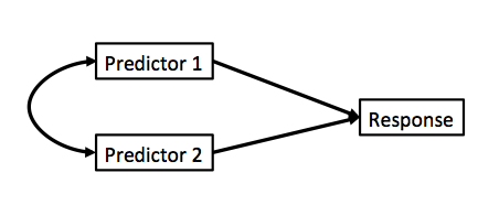![:scale 60%](./images/23/regression2.png) ]

- Curved double-headed arrow indicates COVARIANCE between predictors that we account for.

- We estimate the effect of each predictor **controlling** for all others.  
  
- Can be continous or categorical predictors

---
# We Commonly Encounter Multiple Predictors in Randomized Controlled Blocked Designs
.center[ 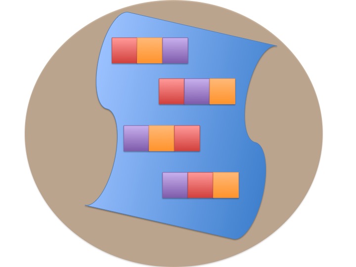![:scale 70%](./images/21/blocked_designs/Slide4.jpg) ]

---
# An Experiment with Orthogonal Treatments: A Graphical View

.center[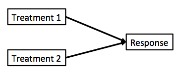![:scale 60%](./images/23/anova.png)]

- This is convenient for estimation

- Observational data is not always so nice, which is OK!

---
# Effects of Stickleback Density on Zooplankton
<br><br>
.pull-left[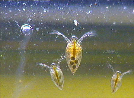![](./images/21/daphnia.jpeg)]
.pull-right[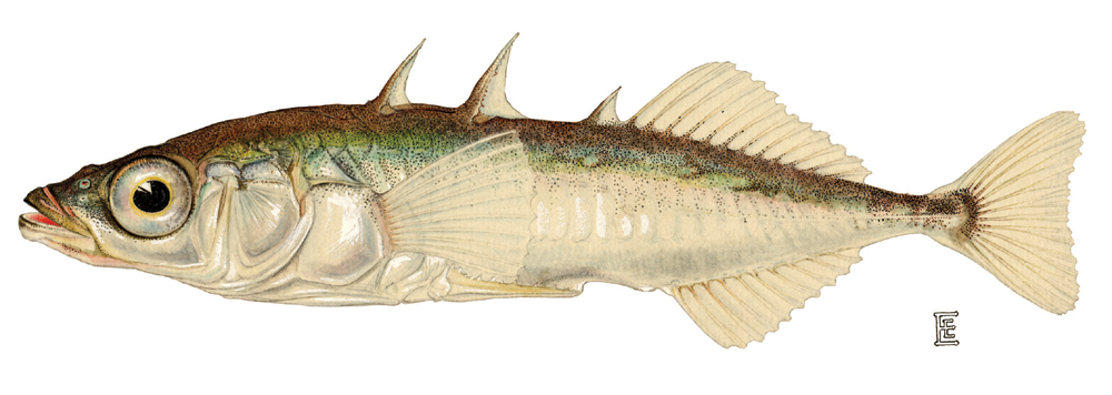![](./images/21/threespine_stickleback.jpeg)]  
   
   
.bottom[Units placed across a lake so that 1 set of each treatment was ’blocked’ together]

---
# Treatment and Block Effects

---
# Multiway Categorical Model
- Many different treatment types  
     - 2-Way is for Treatment and block
     - 3-Way for, e.g., Sticklebacks, Nutrients, and block
     - 4-way, etc., all possible

- For experiments, we assume treatments are fully orthogonal  
      - Each type of treatment type A has all levels of treatment type B
      - E.g., Each stickleback treatment is present in each block

- Experiment is **balanced** for **simple effects**  
      - Simple effect is the unique combination of two or more treatments  
      - Balance implies the sample size for each treatment combination is the same 
      - But, hey, this is more for inference, rather than **estimation**

---
# Fitting a Model with Mutiple Categorical Predictors

```r
zoop_lm <- lm(zooplankton ~ treatment + 
                block, data=zoop)

zoop_lm
```

```

Call:
lm(formula = zooplankton ~ treatment + block, data = zoop)

Coefficients:
  (Intercept)  treatmenthigh   treatmentlow         block2         block3  
     3.42e+00      -1.64e+00      -1.02e+00       9.57e-16      -7.00e-01  
       block4         block5  
    -1.00e+00      -3.00e-01  
```

--
 Note the treatment contrasts!

---
# Assumptions of Categorical Models with Many Categories
-   Independence of data points

-   No relationship between fitted and residual values  
     - .red[ Additivity (linearity) of Treatments ]
  
-   Normality within groups (of residuals)  
  
-   Homoscedasticity (homogeneity of variance) of groups  
  
- No *collinearity* between levels of different categories

---
# The Usual on Predictions
<img src="many_types_of_predictors_files/figure-html/unnamed-chunk-2-1.png" style="display: block; margin: auto;" />

---
# Linearity (and additivity!)
<img src="many_types_of_predictors_files/figure-html/unnamed-chunk-3-1.png" style="display: block; margin: auto;" />

---
# What is Non-Additivity?
The effect of category depends on another - e.g. this grazing experiment

---
# Non-Additivity is Parabolic

---
class: center, middle

![](images/many_predictors/bad_model.jpg)

---
# Normality!

---
# HOV!

---
# Collinearity!
<img src="many_types_of_predictors_files/figure-html/unnamed-chunk-8-1.png" style="display: block; margin: auto;" />

- by definition, not a problem in an experiment

---
# How do We Understand the Modeled Results?

- Coefficients (but treatment contrasts)  
  
  
- Expected means of levels of each category
     - Average over other categories
  
  
- Differences between levels of each category

---
# Coefficients and Treatment Contrasts

<table class="table" style="margin-left: auto; margin-right: auto;">
 <thead>
  <tr>
   <th style="text-align:left;"> term </th>
   <th style="text-align:right;"> estimate </th>
   <th style="text-align:right;"> std.error </th>
  </tr>
 </thead>
<tbody>
  <tr>
   <td style="text-align:left;"> (Intercept) </td>
   <td style="text-align:right;"> 3.42 </td>
   <td style="text-align:right;"> 0.31 </td>
  </tr>
  <tr>
   <td style="text-align:left;"> treatmenthigh </td>
   <td style="text-align:right;"> -1.64 </td>
   <td style="text-align:right;"> 0.29 </td>
  </tr>
  <tr>
   <td style="text-align:left;"> treatmentlow </td>
   <td style="text-align:right;"> -1.02 </td>
   <td style="text-align:right;"> 0.29 </td>
  </tr>
  <tr>
   <td style="text-align:left;"> block2 </td>
   <td style="text-align:right;"> 0.00 </td>
   <td style="text-align:right;"> 0.37 </td>
  </tr>
  <tr>
   <td style="text-align:left;"> block3 </td>
   <td style="text-align:right;"> -0.70 </td>
   <td style="text-align:right;"> 0.37 </td>
  </tr>
  <tr>
   <td style="text-align:left;"> block4 </td>
   <td style="text-align:right;"> -1.00 </td>
   <td style="text-align:right;"> 0.37 </td>
  </tr>
  <tr>
   <td style="text-align:left;"> block5 </td>
   <td style="text-align:right;"> -0.30 </td>
   <td style="text-align:right;"> 0.37 </td>
  </tr>
</tbody>
</table>

- Intercept is block 1, treatment control  
  
- Other coefs are all deviation from control in block 1

---
# Means Averaging Over Other Category

```
 treatment emmean    SE df lower.CL upper.CL
 control     3.02 0.205  8    2.548     3.49
 high        1.38 0.205  8    0.908     1.85
 low         2.00 0.205  8    1.528     2.47

Results are averaged over the levels of: block 
Confidence level used: 0.95 
```

```
 block emmean    SE df lower.CL upper.CL
 1       2.53 0.264  8    1.924     3.14
 2       2.53 0.264  8    1.924     3.14
 3       1.83 0.264  8    1.224     2.44
 4       1.53 0.264  8    0.924     2.14
 5       2.23 0.264  8    1.624     2.84

Results are averaged over the levels of: treatment 
Confidence level used: 0.95 
```

---
# Visualize the Expected Means

---
# Differences Between Treatments

```
 contrast       estimate    SE df lower.CL upper.CL
 control - high     1.64 0.289  8    0.972   2.3075
 control - low      1.02 0.289  8    0.352   1.6875
 high - low        -0.62 0.289  8   -1.288   0.0475

Results are averaged over the levels of: block 
Confidence level used: 0.95 
```

---
# Many Additive Predictors

1.   Multiple Linear Regression

2.   Many Categories with Many Levels

3.   <font color = "red">Combining Categorical and Continuous Predictors</font>

---
# It's All One

**The Linear Model**
`$$\boldsymbol{Y} = \boldsymbol{b X} + \boldsymbol{\epsilon}$$`

**Multiple Continuous Predictors**
`$$y_{i} = \beta_{0} + \sum \beta_{j}x_{ij} + \epsilon_{i}$$`

**Many Categorical Predictors**
`$$y_{ijk} = \beta_{0} + \sum \beta_{i}x_{ik} + \sum \beta_{j}x_{jk} + \epsilon_{ijk}$$`

---
# Mixing Continuous and Categorical Predictors: Analysis of Covariance

`$$y_{ij} = \beta_0   + \beta_{1}x_{1i} + \sum\beta_j x_{ij} +  + \epsilon_{ij}$$`

$$ x_{ij} = 0,1 \qquad \epsilon \sim \mathcal{N}(0,\sigma)$$

-   Categorical Variable + a continuous predictor  
  
-   Often used to correct for a gradient or some continuous variable affecting outcome  
  
-   OR used to correct a regression due to additional groups that may throw off slope estimates  
      - e.g. Simpson's Paradox: A positive relationship between test scores and academic performance can be masked by gender differences

---
# Simpson's Paradox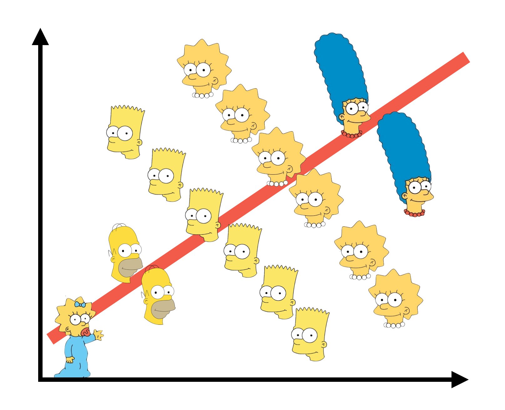
![](./images/many_predictors/simpsons_paradox.jpg)

---
# What is Simpson's Paradox: Penguin Example

---
# What is Simpson's Paradox: Penguin Example

Note: This can happen with just continuous variables as well

---

# Neanderthals and Categorical/Continuous Variables

.center[ ![:scale 60%](./images/23/neanlooking.jpeg) ]

Who had a bigger brain: Neanderthals or us?

---
# The Means Look the Same...

---
# But there appears to be a Relationship Between Body and Brain Mass

---
# And Mean Body Mass is Different

---
class: center, middle 
![](images/23/redo_analysis.jpg)

---
# Categorical Model with a Continuous Covariate for Control

Evaluate a categorical effect(s), controlling for a *covariate* (parallel lines)  
   
Groups modify the *intercept*.

---
# Assumptions are the Same!
  
-   Independence of data points
  
-   Additivity of Treatment and Covariate (Parallel Slopes)  
  
-   Normality and homoscedacticity within groups (of residuals)  
  
-   No relationship between fitted and residual values

---
# Linearity Assumption KEY
<img src="many_types_of_predictors_files/figure-html/zoop_assumptions-1.png" style="display: block; margin: auto;" />

---
# Test for Parallel Slopes
We fit a model where slopes are not parallel:

`$$y_{ijk} = \beta_0 + \beta_{1}x_1  + \sum_{j}^{i=1}\beta_j x_{ij} + \sum_{j}^{i=1}\beta_{k}x_1 x_{ij} + \epsilon_ijk$$`

If you have an interaction, welp, that's a different model - slopes vary by group!

---
# VIF Also *Very* Important
<img src="many_types_of_predictors_files/figure-html/unnamed-chunk-14-1.png" style="display: block; margin: auto;" />

---
# Usual Normality Assumption
<img src="many_types_of_predictors_files/figure-html/unnamed-chunk-15-1.png" style="display: block; margin: auto;" />

---
# Usual HOV Assumption
<img src="many_types_of_predictors_files/figure-html/unnamed-chunk-16-1.png" style="display: block; margin: auto;" />

---
# Usual Outlier Assumption
<img src="many_types_of_predictors_files/figure-html/unnamed-chunk-17-1.png" style="display: block; margin: auto;" />

---
# The Results

- We can look at coefficients  
  
- We can look at means adjusted for covariate   
  
- Visualize! Visualize! Visualize!

---
# Those Coefs

- Intercept is species = neanderthal, but lnmass = 0?  
  
- Categorical coefficient is change in intercept for recent  
  
- lnmass coefficient is change in ln brain mass per change in 1 unit of ln mass

---
# Groups Means at Mean of Covariate
<table class="table" style="margin-left: auto; margin-right: auto;">
 <thead>
  <tr>
   <th style="text-align:left;"> species </th>
   <th style="text-align:right;"> emmean </th>
   <th style="text-align:right;"> SE </th>
   <th style="text-align:right;"> df </th>
   <th style="text-align:right;"> lower.CL </th>
   <th style="text-align:right;"> upper.CL </th>
  </tr>
 </thead>
<tbody>
  <tr>
   <td style="text-align:left;"> neanderthal </td>
   <td style="text-align:right;"> 7.272 </td>
   <td style="text-align:right;"> 0.024 </td>
   <td style="text-align:right;"> 36 </td>
   <td style="text-align:right;"> 7.223 </td>
   <td style="text-align:right;"> 7.321 </td>
  </tr>
  <tr>
   <td style="text-align:left;"> recent </td>
   <td style="text-align:right;"> 7.342 </td>
   <td style="text-align:right;"> 0.013 </td>
   <td style="text-align:right;"> 36 </td>
   <td style="text-align:right;"> 7.317 </td>
   <td style="text-align:right;"> 7.367 </td>
  </tr>
</tbody>
</table>

Can also evaluate for other levels of the covariate as is interesting

---
# We Can Compare Groups Adjusting for Covariates
.center[ ![:scale 60%](./images/many_predictors/bonferroni_meme.jpg) ]

---
# Difference Between Groups at Mean of Covariate
<table class="table" style="margin-left: auto; margin-right: auto;">
 <thead>
  <tr>
   <th style="text-align:left;"> contrast </th>
   <th style="text-align:right;"> estimate </th>
   <th style="text-align:right;"> SE </th>
   <th style="text-align:right;"> df </th>
   <th style="text-align:right;"> lower.CL </th>
   <th style="text-align:right;"> upper.CL </th>
  </tr>
 </thead>
<tbody>
  <tr>
   <td style="text-align:left;"> neanderthal - recent </td>
   <td style="text-align:right;"> -0.07 </td>
   <td style="text-align:right;"> 0.028 </td>
   <td style="text-align:right;"> 36 </td>
   <td style="text-align:right;"> -0.128 </td>
   <td style="text-align:right;"> -0.013 </td>
  </tr>
</tbody>
</table>

---
# Visualizing Result Says it All!
<img src="many_types_of_predictors_files/figure-html/unnamed-chunk-19-1.png" style="display: block; margin: auto;" />

---
# Or Plot at the Mean Level of the Covariate
<img src="many_types_of_predictors_files/figure-html/unnamed-chunk-20-1.png" style="display: block; margin: auto;" />

---
# Extensions of the Linear Additive Model

- Wow, we sure can fit a lot in there!

- Categorical is just continuous as 0/1   
  
- So, we can build a LOT of models, limited only by our imagination!