Linear Models and Frequentist Hypothesis Testing

class: center, middle

# Linear Models and Frequentist Hypothesis Testing
<br>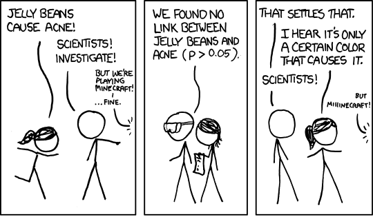
![:scale 75%](images/07/xkcd_sig_blowup.png)
.left[.small[https://xkcd.com/882/]]

---
class: center, middle

# Etherpad
<br><br>
<center><h3>https://etherpad.wikimedia.org/p/607-nht-2023</h3></center>

---

# Up Until Now, I've Shied Away from Inference

<table class=" lightable-classic" style='font-family: "Arial Narrow", "Source Sans Pro", sans-serif; margin-left: auto; margin-right: auto;'>
 <thead>
  <tr>
   <th style="text-align:left;"> term </th>
   <th style="text-align:right;"> estimate </th>
   <th style="text-align:right;"> std.error </th>
  </tr>
 </thead>
<tbody>
  <tr>
   <td style="text-align:left;"> (Intercept) </td>
   <td style="text-align:right;"> 1.92 </td>
   <td style="text-align:right;"> 1.51 </td>
  </tr>
  <tr>
   <td style="text-align:left;"> resemblance </td>
   <td style="text-align:right;"> 2.99 </td>
   <td style="text-align:right;"> 0.57 </td>
  </tr>
</tbody>
</table>

We've talked about effect sizes, confidence intervals as a measure of precision...

---
class: center, middle

# So.... how do you draw conclusions from an experiment or observation?

---
# Inductive v. Deductive Reasoning

<br><br>
**Deductive Inference:** A larger theory is used to devise
many small tests.

**Inductive Inference:** Small pieces of evidence are used
to shape a larger theory and degree of belief.
---

# Applying Different Styles of Inference

- **Null Hypothesis Testing**: What's the probability that things are not influencing our data?
      - Deductive

- **Cross-Validation**: How good are you at predicting new data?
      - Deductive

- **Model Comparison**: Comparison of alternate hypotheses
      - Deductive or Inductive

- **Probabilistic Inference**: What's our degree of belief in a data?
      - Inductive

---

# Testing Our Models

1. How do we Know

2. Evaluating a Null Hypothesis

3. Testing Linear Models

---
# The Core Philosophy of Frequentist Inference and Severe Statistical Testing

- We are estimating the probability of an outcome of an event over the long-term

- Thus, we calculate a **test statistic** based on our **sample** assuming it is representative of a population

- We compare that to the distribution of the test statistic from an assumed population

- We ask, in the long-term, what's the probability of observing our test statistic of a more extreme statistic given our assumed population

---

# R.A. Fisher and The P-Value

.pull-left[
![](./images/07/fisher2.jpeg)
]

.pull-right[
P-value: The Probability of making an observation or more extreme
observation given that the particular hypothesis is true.
]

---
# Putting P-Values Into Practice with Pufferfish

.pull-left[
- Pufferfish are toxic/harmful to predators  
<br>
- Batesian mimics gain protection from predation - why?
<br><br>
- Evolved response to appearance?
<br><br>
- Researchers tested with mimics varying in toxic pufferfish resemblance
]

.pull-right[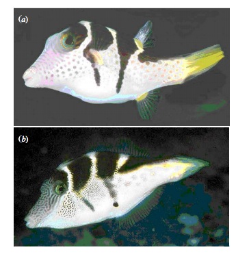
![:scale 80%](./images/11/puffer_mimics.jpg)
]

---
# Does Resembling a Pufferfish Reduce Predator Visits?
<img src="linear_regression_nht_files/figure-html/puffershow-1.png" style="display: block; margin: auto;" />

---

#  What is the probability of a slope of ~3 or greater GIVEN a Hypothesis of a Slope of 2?

We know our SE of our estimate is 0.57, so, we have a distribution of what we **could** observe.

---
#  What is the probability of a slope of ~3 or greater GIVEN a Hypothesis of a Slope of 2?

BUT - our estimated slope is ~3.

---
# To test the 2:1 hypothesis, we need to know the probability of observing 3, or something GREATER than 3.

We want to know if we did this experiment again and again, what's the probability of observing what we saw or worse (frequentist!)

<img src="linear_regression_nht_files/figure-html/add_p-1.png" style="display: block; margin: auto;" />
--

Probability = 0.04

---
# Two-Tails for Testing

We typically look at extremes in both tails to get at "worse" unless we have a directional hypothesis

<img src="linear_regression_nht_files/figure-html/add_p_2-1.png" style="display: block; margin: auto;" />
--

Probability = 0.08

---
# But What does a P-Value MEAN?!?!?!

.center[**The Probability of Observing Your Sample or a More Extreme Sample Given that a Hypothesis is True**]

- It is NOT evidence FOR the hypothesis

- It is evidence AGAINST the hypothesis

- It is not conclusive - it's value depends on study design

---
# For Example, Sample Size
Difference between groups = 0.1, sd = 0.5, Hypothesis: Difference Between Groups is 0

---

# How Does a P-Value Work with Respect to Inference?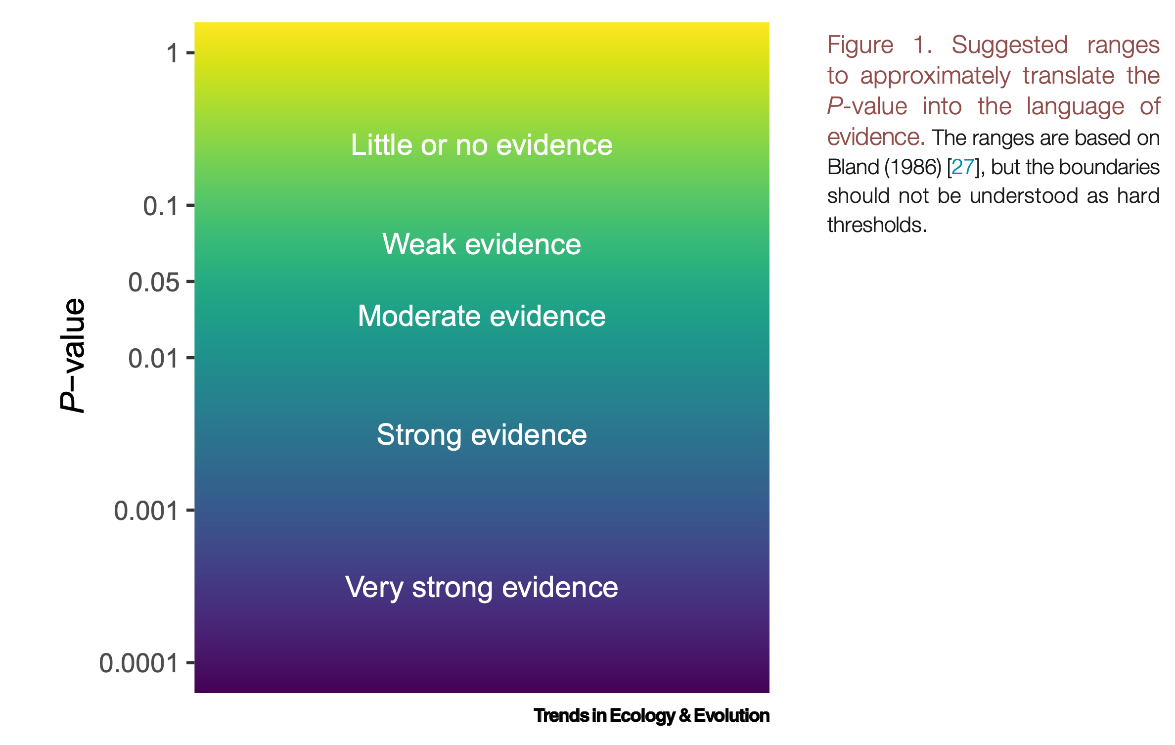

![](images/nht/muff_et_al_2022_pvalue.png)
Muff et al. 2022 TREE

---

# Testing Our Models

1. How do we Know

2. .red[Evaluating a Null Hypothesis.]

3. Testing Linear Models

---
# Null Hypothesis Testing is a Form of Deductive Inference

.pull-left[
![:scale 55%](./images/07/Karl_Popper_wikipedia.jpeg)

Falsification of hypotheses is key! <br><br>

A theory should be considered scientific if, and only if, it is falsifiable.

]

--
.pull-right[
![:scale 55%](./images/regression/Professor_Imre_Lakatos,_c1960s.jpg)

Look at a whole research program and falsify auxilliary hypotheses
]

---
# A Bigger View of Dedictive Inference

![](./images/regression/lakatos_structure.png)

.small[https://plato.stanford.edu/entries/lakatos/#ImprPoppScie]

---
class: center, middle

# Null hypothesis testing is asking what is the probability of our observation or more extreme observation given that some **null expectation** is true.

### (it is .red[**NOT**] the probability of any particular alternate hypothesis being true)

---
# Applying Fisherian P-Values: Evaluation of a Test Statistic

We  use our data to calculate a **test statistic** that maps to a value
of the null distribution.

We can then calculate the probability of observing our data, or of observing data even more extreme, given that the null hypothesis is true.

`$$\large P(X \leq Data | H_{0})$$`

---
# Problems with P

- Most people don't understand it.
     - See American Statistical Society' recent statements

- We don't know how to talk about it

- Interpretation of P-values as confirmation of an alternative hypothesis
     
--

- Like SE, it gets smaller with sample size!

- Misuse of setting a threshold for rejecting a hypothesis

---

# How Should We Evaluate NHT P-Values?

![](images/nht/muff_et_al_2022_pvalue.png)
Muff et al. 2022 TREE

---
# Neyman-Pearson Hypothesis Testing and Decision Making: What if you have to make a choice?

.pull-left[ 
![image](./images/08/neyman.jpeg)

Jerzy Neyman
]

.pull-right[
![image](./images/08/Pearson_Egon_4.jpeg)

Egon Pearson
]

---
# Neyman-Pearson Null Hypothesis Significance Testing

- For Industrial Quality Control, NHST was introduced to establish cutoffs of reasonable p, called an `$\alpha$`

- This corresponds to Confidence intervals: 1 - `$\alpha$` = CI of interest

- Results with p `$\le$` `$\alpha$` are deemed **statistically significant**

---

# NHST in a nutshell

1. Establish a critical threshold below which one rejects a null hypothesis - `$\alpha$`\. *A priori* reasoning sets this threshold.

2. Neyman and Pearon state that if p `$\le$` `$\alpha$` then we reject the null. 
     - Think about this in a quality control setting - it's GREAT!  
--

3. Fisher suggested a typical `$\alpha$` of 0.05 as indicating **statistical significance**, although eschewed the idea of a decision procedure where a null is abandoned. 
    - Codified by the FDA for testing!

4. This has become weaponized so that `$\alpha = 0.05$` has become a norm.... and often determines if something is worthy of being published?
     
---
class: center, middle

.center[
# AND... Statistical Significance is NOT Biological Signficance.
]

---

# Why 0.05? Remember, 2SD = 95% CI

> **It is convenient** to take this point as a limit in judging whether a deviation is to be considered significant or not. Deviations exceeding twice the standard deviation are thus formally regarded as significant

Fisher, R.A. (1925) Statistical Methods for Research Workers, p. 47

---

# But Even Fisher Argued for Situational `$\alpha$`

>If one in twenty does not seem high enough odds, we may, if we prefer it, draw the line at one in fifty (the 2 per cent point), or one in a hundred (the 1 per cent point). Personally, the writer prefers to set a low standard of significance at the 5 per cent point, and ignore entirely all results which fail to reach this level. A scientific fact should be regarded as experimentally established only if a properly designed experiment rarely fails to give this level of significance.

Fisher, R.A. (1926) The arrangement of field experiments.
 Journal of the Ministry of Agriculture, p. 504

---
# And, Really, All of This is Just Fisher Dodging Royalty Payments

> We were surprised to learn, in the course of writing this article, that the p<0.05 cutoff was established as a competitive response to a disagreement over book royalties between two foundational statisticians.

> In the early 1920s, Kendall Pearson ... whose income depended on the sale of extensive statistical tables, was unwilling to allow Ronald A. Fisher to use them in his new book. To work around this barrier, Fisher created a method of inference based on only two values: p-values of 0.05 and 0.01.

from Brent Goldfarb and Andrew W. King. "Scientific Apophenia in Strategic Management Research: Significance & Mistaken Inference." Strategic Management Journal, vol. 37, no. 1, Wiley, 2016, pp. 167–76.

---
# And really, what does p = 0.061 mean?

- There is a 6.1% chance of obtaining the observed data or more extreme data given that the null hypothesis is true.

- If you choose to reject the null, you have a ~ 1 in 16 chance of being wrong

- Are you comfortable with that?

- OR - What other evidence would you need to make you more or less comfortable?

---
# How do you talk about results from a p-value?

- Based on your experimental design, what is a reasonable range of p-values to expect if the null is false

- Smaller p values indicate stronger support for rejection, larger ones weaker. Use that language! Not significance!

- Accumulate multiple lines of evidence so that the entire edifice of your research does not rest on a single p-value!!!!

---
# How I talk about p-values

- At different p-values, based on your study design, you will have different levels of confidence about rejecting your null. For example, based on the design of one study...

- A p value of less than 0.0001 means I have very high confidence in rejecting the null

- A p-value of 0.01 means I have high confidence in rejecting the null

- A p-value between 0.05 and 0.1 means I have some confidence in rejecting the null

- A p-value of > 0.1 means I have low confidence in rejecting the null

---
# My Guiding Light (alongside Muff et al. 2022)

.center[
![](./images/15/ipcc_uncertainty_ar5.jpg)
]

---

# Testing Our Models

1. How do we Know

2. Evaluating a Null Hypothesis.

3. .red[Testing Linear Models]

---

# Common Regression Test Statistics

- Are my coefficients 0?
    - **Null Hypothesis**: Coefficients are 0  
    - **Test Statistic**: T distribution (normal distribution modified for low sample size)

- Does my model explain variability in the data?
     - **Null Hypothesis**: The ratio of variability from your predictors versus noise is 1
     - **Test Statistic**: F distribution (describes ratio of two variances)

---
background-image: url(images/09/guiness_full.jpg)
background-position: center
background-size: contain
background-color: black

---
background-image: url(images/09/gosset.jpg)
background-position: center
background-size: contain

---
# T-Distributions are What You'd Expect Sampling a Standard Normal Population with a Small Sample Size

- t = mean/SE, DF = n-1
- It assumes a normal population with mean of 0 and SD of 1

---
# Assessing the Slope with a T-Test
<br>
`$$\Large t_{b} = \frac{b - \beta_{0}}{SE_{b}}$$`

#### DF=n-2

`$H_0: \beta_{0} = 0$`, but we can test other hypotheses

---
# Slope of Puffer Relationship (DF = 1 for Parameter Tests)
<table>
 <thead>
  <tr>
   <th style="text-align:left;">   </th>
   <th style="text-align:right;"> Estimate </th>
   <th style="text-align:right;"> Std. Error </th>
   <th style="text-align:right;"> t value </th>
   <th style="text-align:right;"> Pr(&gt;|t|) </th>
  </tr>
 </thead>
<tbody>
  <tr>
   <td style="text-align:left;"> (Intercept) </td>
   <td style="text-align:right;"> 1.925 </td>
   <td style="text-align:right;"> 1.506 </td>
   <td style="text-align:right;"> 1.278 </td>
   <td style="text-align:right;"> 0.218 </td>
  </tr>
  <tr>
   <td style="text-align:left;"> resemblance </td>
   <td style="text-align:right;"> 2.989 </td>
   <td style="text-align:right;"> 0.571 </td>
   <td style="text-align:right;"> 5.232 </td>
   <td style="text-align:right;"> 0.000 </td>
  </tr>
</tbody>
</table>

<Br>
p is **very** small here so...  
We reject the hypothesis of no slope for resemblance, but fail to reject it for the intercept.

---

# So, what can we say in a null hypothesis testing framework?

.pull-left[

- We reject that there is no relationship between resemblance and predator visits in our experiment.

- 0.6 of the variability in predator visits is associated with resemblance. 
]

.pull-right[

<img src="linear_regression_nht_files/figure-html/puffershow-1.png" style="display: block; margin: auto;" />
]

---
# Does my model explain variability in the data?

Ho = The model predicts no variation in the data.

Ha = The model predicts variation in the data.

To evaluate these hypotheses, we need to have a measure of variation explained by data versus error - the sums of squares!

This is an Analysis of Variance..... **ANOVA**!

--
`$$SS_{Total} = SS_{Regression} + SS_{Error}$$`
---

# Sums of Squares of Error, Visually
<img src="linear_regression_nht_files/figure-html/linefit-1.png" style="display: block; margin: auto;" />

---
# Sums of Squares of Regression, Visually
<img src="linear_regression_nht_files/figure-html/ssr-1.png" style="display: block; margin: auto;" />

Distance from `$\hat{y}$` to `$\bar{y}$`

---
# Components of the Total Sums of Squares

`$SS_{R} = \sum(\hat{Y_{i}} - \bar{Y})^{2}$`, df=1

`$SS_{E} = \sum(Y_{i} - \hat{Y}_{i})^2$`, df=n-2

--
To compare them, we need to correct for different DF. This is the Mean
Square.

MS=SS/DF

e.g, `$MS_{E} = \frac{SS_{E}}{n-2}$`

---

# The F Distribution and Ratios of Variances

`$F = \frac{MS_{R}}{MS_{E}}$` with DF=1,n-2

---
# F-Test and Pufferfish
<table>
 <thead>
  <tr>
   <th style="text-align:left;">   </th>
   <th style="text-align:right;"> Df </th>
   <th style="text-align:right;"> Sum Sq </th>
   <th style="text-align:right;"> Mean Sq </th>
   <th style="text-align:right;"> F value </th>
   <th style="text-align:right;"> Pr(&gt;F) </th>
  </tr>
 </thead>
<tbody>
  <tr>
   <td style="text-align:left;"> resemblance </td>
   <td style="text-align:right;"> 1 </td>
   <td style="text-align:right;"> 255.1532 </td>
   <td style="text-align:right;"> 255.153152 </td>
   <td style="text-align:right;"> 27.37094 </td>
   <td style="text-align:right;"> 5.64e-05 </td>
  </tr>
  <tr>
   <td style="text-align:left;"> Residuals </td>
   <td style="text-align:right;"> 18 </td>
   <td style="text-align:right;"> 167.7968 </td>
   <td style="text-align:right;"> 9.322047 </td>
   <td style="text-align:right;"> NA </td>
   <td style="text-align:right;"> NA </td>
  </tr>
</tbody>
</table>

<br><br>
--
We  reject the null hypothesis that resemblance does not explain variability in predator approaches

---
# Testing the Coefficients

-  F-Tests evaluate whether elements of the model contribute to variability in the data
      - Are modeled predictors just noise?
      - What's the difference between a model with only an intercept and an intercept and slope?

- T-tests evaluate whether coefficients are different from 0

- Often, F and T agree - but not always
    - T can be more sensitive with multiple predictors

---

# What About Models with Categorical Variables?

- T-tests for Coefficients with Treatment Contrasts

- F Tests for Variability Explained by Including Categorical Predictor  
      - **ANOVA**
  
- More T-Tests for Posthoc Evaluation

---
# What Explains This Data? Same as Regression (because it's all a linear model)
<img src="linear_regression_nht_files/figure-html/brain_anova_viz_1-1.png" style="display: block; margin: auto;" />

---
# Variability due to Model (between groups)
<img src="linear_regression_nht_files/figure-html/brain_anova_viz_2-1.png" style="display: block; margin: auto;" />

---
# Variability due to Error (Within Groups)
<img src="linear_regression_nht_files/figure-html/brain_anova_viz_3-1.png" style="display: block; margin: auto;" />

---
# F-Test to Compare
<br><br>
`$SS_{Total} = SS_{Model} + SS_{Error}$`

(Classic ANOVA: `$SS_{Total} = SS_{Between} + SS_{Within}$`)

Yes, these are the same!

---
# F-Test to Compare

`$SS_{Model} = \sum_{i}\sum_{j}(\bar{Y_{i}} - \bar{Y})^{2}$`, df=k-1

`$SS_{Error} = \sum_{i}\sum_{j}(Y_{ij} - \bar{Y_{i}})^2$`, df=n-k

To compare them, we need to correct for different DF. This is the Mean Square.

MS = SS/DF, e.g, `$MS_{W} = \frac{SS_{W}}{n-k}$`

---
# ANOVA

<table>
 <thead>
  <tr>
   <th style="text-align:left;">   </th>
   <th style="text-align:right;"> Df </th>
   <th style="text-align:right;"> Sum Sq </th>
   <th style="text-align:right;"> Mean Sq </th>
   <th style="text-align:right;"> F value </th>
   <th style="text-align:right;"> Pr(&gt;F) </th>
  </tr>
 </thead>
<tbody>
  <tr>
   <td style="text-align:left;"> group </td>
   <td style="text-align:right;"> 2 </td>
   <td style="text-align:right;"> 0.5402533 </td>
   <td style="text-align:right;"> 0.2701267 </td>
   <td style="text-align:right;"> 7.823136 </td>
   <td style="text-align:right;"> 0.0012943 </td>
  </tr>
  <tr>
   <td style="text-align:left;"> Residuals </td>
   <td style="text-align:right;"> 42 </td>
   <td style="text-align:right;"> 1.4502267 </td>
   <td style="text-align:right;"> 0.0345292 </td>
   <td style="text-align:right;"> NA </td>
   <td style="text-align:right;"> NA </td>
  </tr>
</tbody>
</table>

We have strong confidence that we can reject the null hypothesis

---
# This Works the Same for Multiple Categorical

TreatmentHo: `$\mu_{i1} = \mu{i2} = \mu{i3} = ...$`

Block Ho: `$\mu_{j1} = \mu{j2} = \mu{j3} = ...$`

i.e., The variance due to each treatment type is no different than noise

---
# We Decompose Sums of Squares for Multiple Predictors

`$SS_{Total} = SS_{A} + SS_{B} + SS_{Error}$`

- Factors are Orthogonal and Balanced, so, Model SS can be split
     -   F-Test using Mean Squares as Before

---

# What About Unbalanced Data or Mixing in Continuous Predictors?

- Let's Assume Y ~ A + B where A is categorical and B is continuous

- F-Tests are really model comparisons

- The SS for A is the Residual SS of Y ~ A + B  - Residual SS of Y ~ B 
      - This type of SS is called **marginal SS** or **type II SS**
      
--

- Proceed as normal

- This also works for interactions, where interactions are all tested including additive or lower-level interaction components
     - e.g., SS for AB is RSS for A+B+AB - RSS for A+B
     
---

# Warning for Working with SAS Product Users (e.g., JMP)

- You will sometimes see *Type III* which is sometimes nonsensical
     - e.g., SS for A is RSS for A+B+AB - RSS for B+AB
     
--

- Always question the default settings!

---
class:center, middle

# F-Tests tell you if you can reject the null that predictors do not explain anything

---
# Post-Hoc Comparisons of Groups

- **Only compare groups if you reject a Null Hypothesis via F-Test**
      - Otherwise, any results are spurious  
      - This is why they are called post-hocs
      
--

- We've been here before with SEs and CIs

- In truth, we are using T-tests

- BUT - we now correct p-values for Family-Wise Error (if at all)

---

![](images/nht/princess_bride_significant.png)