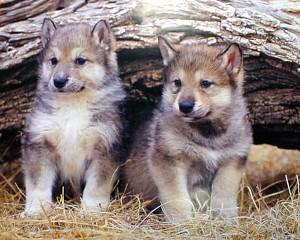
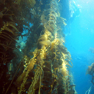
Generalized Linear Models and Overdispersion

class: center, middle

# Generalized Linear Models and Overdispersion
 
![:scale 75%](images/glm/name_five_analyses.jpg)

---
# A Generalized Linear World
  
1. How do we fit this: Likelihood

2. Count Data and GLMs

3. Overdispersion

---
class: middle, left

# Likelihood: how well data support a given hypothesis.

--
<br><br><br>

### Note: Each and every parameter choice IS a hypothesis</span></h4>

---
## Likelihood Defined
<br><br>
`$$\Large L(H | D) = p(D | H)$$`

Where the D is the data and H is the hypothesis (model) including a both a data generating process with some choice of parameters (often called `$\theta$`). The error generating process is inherent in the choice of probability distribution used for calculation.

---
## Example of Maximum Likelihood Fit

Let’s say we have counted 10 individuals in a plot. Given that the
population is Poisson distributed, what is the value of `$\lambda$`?

</div>

<div id="right", style="width:40%">
<br><br>
`$$p(x) = \frac{\lambda^{x}e^{-\lambda}}{x!}$$` 
<br>where we search all possible values of &lambda;
</div>

---
## Likelihood Function

`$$\Large p(x) = \frac{\lambda^{x}e^{-\lambda}}{x!}$$` 
<br><br>

- This is a **Likelihood Function** for one sample 
     - It is the Poisson Probability Density function

- `$Dpois = \frac{\lambda^{x}e^{-\lambda}}{x!}$`

---
## What is the probability of many data points given a parameter?

</div>

<div id="right", style="width:40%">
<br><br>
p(a and b) = p(a)p(b)  
<br><br><br>
`$$p(D | \theta) = \prod_{i=1}^n p(d_{i} | \theta)$$`
<br><br>
<span class="fragment">$$    = \prod_{i=1}^n \frac{\theta^{x_i}e^{-\theta}}{x_!}$$</span>
</div>

---

## Can Compare p(data | H) for alternate Parameter Values

Compare `$p(D|\theta_{1})$` versus `$p(D|\theta_{2})$`, choose the one with higher likelihood

---
# In Practice We Use Log-Likelihood Surfaces for Computation and Shape to find the Maximum Likelihood
## (Or Really, Deviance, -2 LL, for optimization)

---
## Optimizing over Multiple Parameters get's Harder

Want to find the Maximum Likelihood (or minimum Deviance) to get the MLE (Maximum Likelihood Estimate) of parameters
---

## Contour Plot of a Likelihood Surface
<img src="glm_overdispersion_files/figure-html/contour_LL-1.png" style="display: block; margin: auto;" />

---

## Issues with Likelihood and Models

1.  What Values Are Used for 95% CI?

2.  Grid Sampling Becomes Slow

3.  Algorithmic Solutions Necessary

4.  Specification of Likelihood Function Unwieldy

---
## Likelihood Profile of One Coefficient Along ML Estimates of the Other
<font color="red">Mean profile</font>, <font color="blue">SD Profile</font>

---
## Then Use Likelihood Profiles to get CIs (more on this later)

```
        2.5 %   97.5 %
mean 3704.364 3756.122
sd   1275.384 1311.887
```

---

## How Do We Search Multiparameter Likelihood Space?

We use <span style="color:red">Algorithms</span>

-   Newtown-Raphson (algorithmicly implemented in <span>nlm</span> and
    <span>BFGS</span> method) uses derivatives
     - good for smooth surfaces & good start values

-   Nelder-Mead Simplex (<span>optim</span>’s default)
     - good for rougher surfaces, but slower

-   Simulated Annealing (<span>SANN</span>) uses Metropolis Algorithm search
     - global solution, but slow

- For GLMs, we use **Iteratively Reweighted Lease Squares**
     - fast
     - specific to models from the exponential family

---
# A Generalized Linear World
  
1. How do we fit this: Likelihood

2. .red[Count Data and GLMs]

3. Overdispersion

---

# Remember our Wolves?

.pull-left[

]

.pull-right[

<br><br>
![](./images/11/CUTE_WOLF_PUPS_by_horsesrock44.jpeg)
]

---

# We Had to Log Transform The Count of Pups

`$$log(y_i) = \beta_0 + \beta_1 x_i + \epsilon_i$$`
  - using count data  
  - relationship is curved
  - cannot have negative pups 
  
<img src="glm_overdispersion_files/figure-html/logplot-1.png" style="display: block; margin: auto;" />

---
# But...

![](images/glm/do_not_log.png)

Note, there is a healthy back-and-forth about this paper in the literature... but I think it has some REALLY good points

---
# Why? Count Data is Discrete - so we need an appropriate distribution
### Enter the Poisson!

In a Poisson, Variance = Mean

---
# The Poisson Generalized Linear Model with its Canonical Link

$$\Large \boldsymbol{\eta_{i}} = \boldsymbol{\beta X_i} $$ 
<br><br>

`$$\Large log(\hat{Y_i}) = \eta_{i}$$`
<br><br>

`$$\Large Y_i \sim \mathcal{P}(\hat{Y_i})$$`

---
# Wait - isn't this just a log transform?

--
No.
--

`$$\Large \boldsymbol{log(Y_{i})} = \boldsymbol{\beta X_i} + \boldsymbol{\epsilon_i}$$` 
implies...
 
--
`$$\Large \boldsymbol{Y_{i}} = e^{\boldsymbol{\beta X_i} + \boldsymbol{\epsilon_i}}$$`
--

This is multiplicative error!

We want additive error - which we get from a GLM with a log link:

`$$\Large y = e^{\beta X} + \epsilon$$`

---
# The Code Matches the Model

```r
wolves_glm <- glm(pups ~ inbreeding.coefficient, 
                  
                  family = poisson(link = "log"),
                  
                  data = wolves)
```

--
Compare to...

```r
wolves_lm <- lm(log(pups) ~ inbreeding.coefficient, 
                  
                  data = wolves)
```

---
# We Still Check Some of the Same Assumptions
<img src="glm_overdispersion_files/figure-html/unnamed-chunk-5-1.png" style="display: block; margin: auto;" />

---
# But Now Quantile Residuals Help Assessment
<img src="glm_overdispersion_files/figure-html/unnamed-chunk-6-1.png" style="display: block; margin: auto;" />

---

# Coefficients... Here Have the Same Meaning as a Log-Normal Model
<table class="table" style="margin-left: auto; margin-right: auto;">
 <thead>
  <tr>
   <th style="text-align:left;"> term </th>
   <th style="text-align:right;"> estimate </th>
   <th style="text-align:right;"> std.error </th>
  </tr>
 </thead>
<tbody>
  <tr>
   <td style="text-align:left;"> (Intercept) </td>
   <td style="text-align:right;"> 1.946 </td>
   <td style="text-align:right;"> 0.220 </td>
  </tr>
  <tr>
   <td style="text-align:left;"> inbreeding.coefficient </td>
   <td style="text-align:right;"> -2.656 </td>
   <td style="text-align:right;"> 0.969 </td>
  </tr>
</tbody>
</table>

- If inbreeding is 0, there are ~ 7 pups ( `$e^{1.946}$` )

- An increase in 1 unit of inbreeding is a ~93% loss in # of pups
      - `$1-e^{-2.656}$`

---
# Did it make a difference?

---
# A Generalized Linear World
  
1. How do we fit this: Likelihood  
  
2. Count Data and GLMs

3. .red[Overdispersion]

---
# What is the relationship between kelp holdfast size and number of fronds?
  
  .center[ ![](images/25/Giant_kelp_adult.jpeg) ]

---
# What About Kelp Holdfasts?
<img src="glm_overdispersion_files/figure-html/kelp-1.png" style="display: block; margin: auto;" />
---
# If you had Tried a Linear Model

```r
kelp_lm <- lm(FRONDS ~ HLD_DIAM, data=kelp)
```

---
# What is our data and error generating process?
<img src="glm_overdispersion_files/figure-html/kelp-1.png" style="display: block; margin: auto;" />

---
# What is our data and error generating process?
  - Data generating process should be exponential
- No values less than 1

--
  
  - Error generating process should be Poisson
- Count data

---
# Let's Fit a Model!

```r
kelp_glm <- glm(FRONDS ~ HLD_DIAM, data=kelp,
                family=poisson(link="log"))
```

---
# Quantile Residuals for Kelp GLM with Log Link
<img src="glm_overdispersion_files/figure-html/kelp_resid_dharma-1.png" style="display: block; margin: auto;" />

---
# Ruh Roh! What happened? Overdispersion of Data!

- When the variance increases faster than it should from a model, your data is overdispersed 
     - Underdispersion is also possible

--
  
- This can be solved with different distributions whose variance have different properties  
  
--
  
- OR, we can fit a model, then scale it’s variance posthoc with a coefficient

--
  
-  The likelihood of these latter models is called a Quasi-likelihood, as it does not reflect the true spread of the data  
     - Good to avoid, as it causes inferential difficulties down the line

---
# For Count Data, Two Common Solutions
  
1) Negative Binomial
- Variance = `$\hat{Y_i}^2 + \theta\hat{Y_i}^2$`|$
   - Increases with the square, not linearly
- Although some forms also do linear...  
- Common for **clumped data**  
  
--
  
2) Quasi-Poisson  
- Basically, Variance = `$\theta\hat{Y}$`  
- Posthoc estimation of `$\theta$`
- (Also a similar quasibinomial)

--
  
3) Others where you model dispersion explicitly
- You are in deeper waters here

---
# Plot of Smoothed Residuals v. Predictor
Linear: Quasipoisson, Squared: Negative Binomial

See Ver Hoef and Boveng 2007

---
# New Fits
  
Negative Binomial

```r
library(MASS)
kelp_glm_nb <- glm.nb(FRONDS ~ HLD_DIAM, data=kelp)
```

Quasipoisson

```r
kelp_glm_qp <- glm(FRONDS ~ HLD_DIAM, data=kelp, 
                   family=quasipoisson(link="log"))
```

---
# Checking The Quantile Residuals
  
<img src="glm_overdispersion_files/figure-html/unnamed-chunk-10-1.png" style="display: block; margin: auto;" />

---
# Looks Good!
  
<img src="glm_overdispersion_files/figure-html/unnamed-chunk-11-1.png" style="display: block; margin: auto;" />

---
# What if Fronds Had Been Continuous and We Wanted to Model Overdispersion?

- Can Use a continuous distribution with overdispersion
     - Gamma
     - Variance is `$\hat{Y_i}^2$`
     
- Can model the overdispersion
     - `$y_i \sim \mathcal{N}(\widehat{y_i}, \sigma^2_i)$`
     - Can be a function of predictors

---
# Gamma
Skewed continuous, variance-mean relationship

.pull-left-small[
![](images/glm/waiting_time.jpg)
]

.pull-right-large[
<img src="glm_overdispersion_files/figure-html/unnamed-chunk-12-1.png" style="display: block; margin: auto;" />
]

---

# Similar to Negative Binomial, So, Does it Blend with a log link?

```r
kelp_gamma <- glm(FRONDS ~ HLD_DIAM,
                     family = Gamma(link = "log"),
                     data = kelp)
```

---

# Or, Modeling Variance

`$$log(\widehat{Y_i}) = \beta X_i$$`
  
`$$Y_i \sim \mathcal{N}(\widehat{Y_i}, \sigma^2_i)$$`
  
  
`$$\sigma^2_i = \gamma X_i$$`
Variance can be **linear** function of predictors, or otherwise

---
# Would simple Scaling the Variance have Worked Here?

```r
kelp_var <- glmmTMB(FRONDS ~ HLD_DIAM,
                
                family = gaussian(link = "log"),
                
                dispformula = ~ HLD_DIAM,
                
                data = kelp)
```

---
# Final Note About GLMs and Overdispersion
### Many Distributions Cannot Handle 0s or 1s
  
<img src="glm_overdispersion_files/figure-html/unnamed-chunk-17-1.png" style="display: block; margin: auto;" />

---
class: center, middle

![](images/25/whalberg_assumptions.jpg)