Generalized Linear Models

class: center, middle
# Generalized Linear Models

![:scale 80%](./images/glm/why_cant_you_be_normal.jpg)

---
background-image:url("images/glm/4_consumers.png")
background-size: contain

---
background-image:url("images/glm/plate.png")
background-size: contain

---
### My Data
<table class=" lightable-paper" style='font-family: "Arial Narrow", arial, helvetica, sans-serif; margin-left: auto; margin-right: auto;'>
 <thead>
  <tr>
   <th style="text-align:right;"> predator_richness </th>
   <th style="text-align:right;"> percent_open </th>
  </tr>
 </thead>
<tbody>
  <tr>
   <td style="text-align:right;"> 1 </td>
   <td style="text-align:right;"> 81 </td>
  </tr>
  <tr>
   <td style="text-align:right;"> 2 </td>
   <td style="text-align:right;"> 100 </td>
  </tr>
  <tr>
   <td style="text-align:right;"> 2 </td>
   <td style="text-align:right;"> 70 </td>
  </tr>
  <tr>
   <td style="text-align:right;"> 1 </td>
   <td style="text-align:right;"> 97 </td>
  </tr>
  <tr>
   <td style="text-align:right;"> 2 </td>
   <td style="text-align:right;"> 58 </td>
  </tr>
  <tr>
   <td style="text-align:right;"> 1 </td>
   <td style="text-align:right;"> 96 </td>
  </tr>
  <tr>
   <td style="text-align:right;"> 4 </td>
   <td style="text-align:right;"> 92 </td>
  </tr>
  <tr>
   <td style="text-align:right;"> 1 </td>
   <td style="text-align:right;"> 83 </td>
  </tr>
  <tr>
   <td style="text-align:right;"> 2 </td>
   <td style="text-align:right;"> 99 </td>
  </tr>
  <tr>
   <td style="text-align:right;"> 2 </td>
   <td style="text-align:right;"> 92 </td>
  </tr>
</tbody>
</table>

---
## So....

---
## That was a Terrible Idea
<img src="generalized_linear_models_files/figure-html/unnamed-chunk-2-1.png" style="display: block; margin: auto;" />

---
## That was a Terrible Idea
<img src="generalized_linear_models_files/figure-html/unnamed-chunk-3-1.png" style="display: block; margin: auto;" />

---
## That was a Terrible Idea
<img src="generalized_linear_models_files/figure-html/unnamed-chunk-4-1.png" style="display: block; margin: auto;" />

---
## Log (and other transformations) are not better
<img src="generalized_linear_models_files/figure-html/unnamed-chunk-5-1.png" style="display: block; margin: auto;" />

---
## The Answer is Not Normal.... or Linear
<img src="generalized_linear_models_files/figure-html/unnamed-chunk-6-1.png" style="display: block; margin: auto;" />

---
class:center, middle

![](images/glm/nonnormal_barbie.jpg)

---
# A Generalized Linear World

1. The Generalized Linear Model 
  
2. Logistic Regression & Assumption Tests 
  
3. Logit Curves with Continuous Data

---
# We Have Lived In a Normal World - Until Now

---
# Gaussian Distributions are Part of a Larger Interconnected Family of Distributions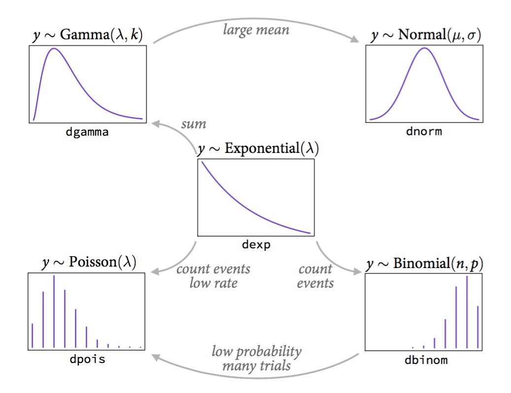

![:scale 90%](images/25/all_dists.jpg)

---
# It Gets Crazy

.center[ 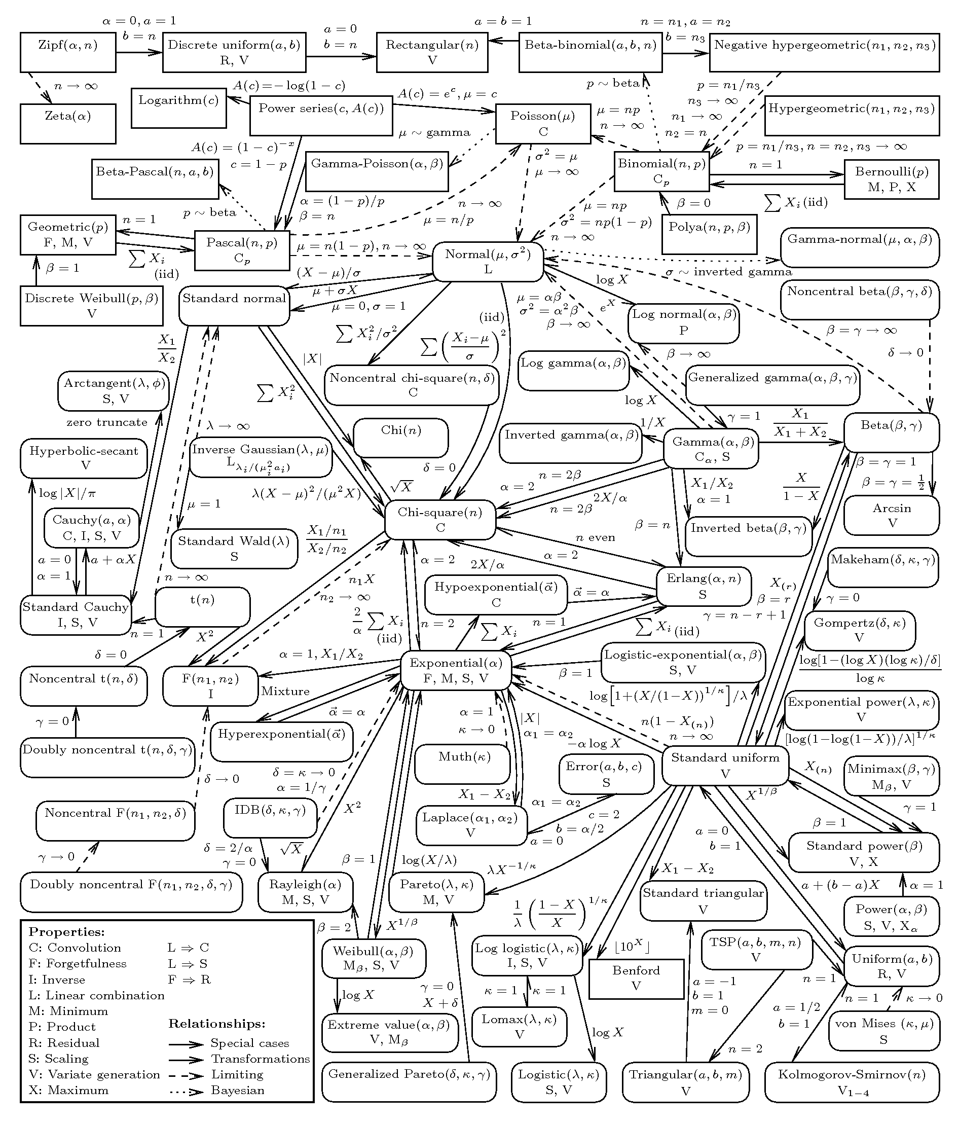![:scale 50%](images/glm/distributions.png) ]

See https://www.randomservices.org/random/special/GeneralExponential.html

---
# The Linear Model with Gaussian Error 
$$\Large \hat{Y_i} = \boldsymbol{\beta X_i} $$ 
<br><br>

`$$\Large Y_i \sim \mathcal{N}(\hat{Y_i},\sigma^{2})$$`

---
# Let's Make a Small Change
$$\Large \boldsymbol{\eta_{i}} = \boldsymbol{\beta X_i} $$ 
<br><br>

`$$\Large \hat{Y_i} = \eta_{i}$$`
<br><br>

`$$\Large Y_i \sim \mathcal{N}(\hat{Y_i},\sigma^{2})$$`

---
# Another Teeeny Change - Link Functions
$$\Large \boldsymbol{\eta_{i}} = \boldsymbol{\beta X_i} $$ 
<br><br>

`$$\Large f(\hat{Y_i}) = \eta_{i}$$`
.red[f is a link function]  
.red[for linear regression, we call this an **identity link**]

`$$\Large Y_i \sim \mathcal{N}(\hat{Y_i},\sigma^{2})$$`

---
## Hold up, isn't this just transformation?

- No.

- `$log(Y) = \beta X + \epsilon$` means that `$Y = exp(\beta X + \epsilon)$`

- A **log link** with a normal residual means that
    - `$log(\widehat{Y}) = \beta X$` but `$\epsilon$` is additive to `$\widehat{Y}$`  
    - SO `$Y = exp(\beta X) + \epsilon$`

---
# So if THIS is the Generalized Linear Model with a Gaussian Error and an Identity Link...
$$\Large \boldsymbol{\eta_{i}} = \boldsymbol{\beta X_i} $$ 
<br><br>

`$$\Large\hat{Y_i} = \eta_{i}$$`

`$$\Large Y_i \sim \mathcal{N}(\hat{Y_i},\sigma^{2})$$`

---
# The Generalized Linear Model
$$\Large \boldsymbol{\eta_{i}} = \boldsymbol{\beta X_i} $$ 
<br><br>

`$$\Large f(\hat{Y_i}) = \eta_{i}$$`
.red[our link doesn't have to be linear]
<br><br>

`$$\Large Y_i \sim \mathcal{D}(\hat{Y_i}, \theta)$$`
<br><br>

`$\mathcal{D}$` is some distribution from the **exponential family**, and `$\theta$` are additional parameters specifying dispersion

---
# What Are Properties of Data that is Not Normal?

- Bounded

- Discrete

- Variance scales with mean

- Skewed, bimodal, or kurtotic

---
class: center, middle

![:scale 80%](images/25/gosling_normality.jpg)

---
# Count Data - Poisson or Negative Binomial
Discrete, variance-mean relationships (linear or squared)

---
# Outcomes of Trials - Binomial
Discrete, Yes/No or # of Outcomes of a Class - we model the probability

.pull-left-small[
![](images/glm/test.jpg)
]

.pull-right-large[
<img src="generalized_linear_models_files/figure-html/unnamed-chunk-10-1.png" style="display: block; margin: auto;" />
]

---
# Time to Achieve Outcomes - Gamma
Skewed continuous, variance-mean relationship

.pull-left-small[
![](images/glm/waiting_time.jpg)
]

.pull-right-large[
<img src="generalized_linear_models_files/figure-html/unnamed-chunk-11-1.png" style="display: block; margin: auto;" />
]
---
# Percents and Porportions - Beta
Bounded, Unimodal to Bimodal

.pull-left-small[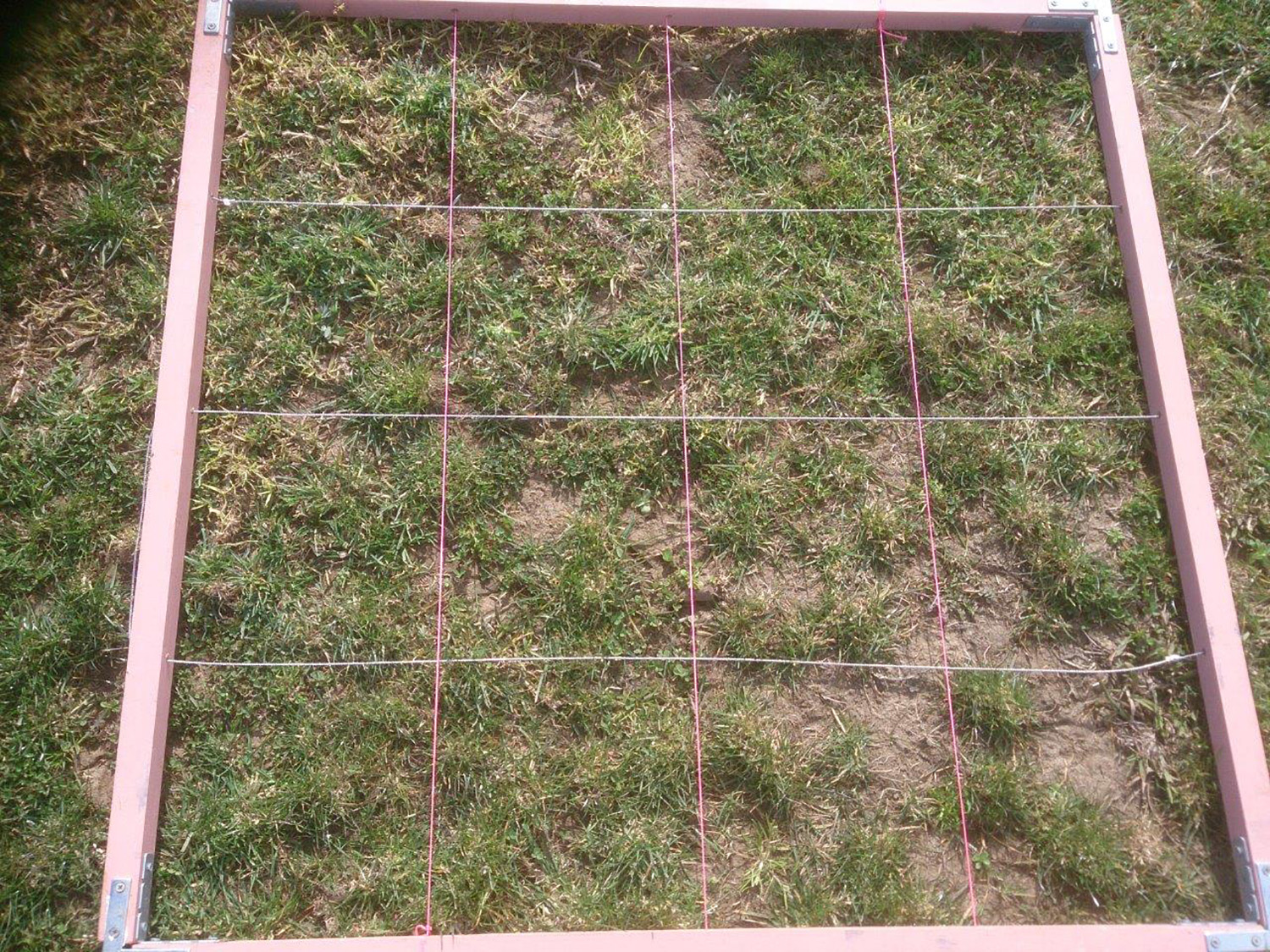
![](images/glm/cover.jpg)
]

.pull-right-large[

]

---
# The Generalized Linear Model
$$\Large \boldsymbol{\eta_{i}} = \boldsymbol{\beta X_i} $$ 
<br><br>

`$$\Large f(\hat{Y_i}) = \eta_{i}$$`
.red[f is a link function]
<br><br>

`$$\Large Y_i \sim \mathcal{D}(\hat{Y_i}, \theta)$$`
<br><br>

`$\mathcal{D}$` is some distribution from the **exponential family**, and `$\theta$` are additional parameters specifying dispersion

---

# Generalized Linear Models: Distributions

1.  The error distribution is from the **exponential family**
  - e.g., Normal, Poisson, Binomial, and more.

2.  For these distributions, the variance is a funciton of the fitted
    value on the curve: `$var(Y_i) = \theta V(\hat{Y_i})$`
  - For a normal distribution, `$var(Y_i) = \theta*1$` as
        `$V(\hat{Y_i})=1$`

- For a poisson distribution, `$var(Y_i) = 1*\mu_i$` as
  `$V(\hat{Y_i})=\hat{Y_i}$`

3. They have *canonical links* which are link functions that fall out from the shape of the distribution and map on to the domain of possible values

- e.g., the identity for the Gaussian  
     
  - We can also use non-canonical links  
        
---
# Distributions, Canonical Links, and Dispersion

|Distribution | Canonical Link | Variance Function|
|-------------|-------------|-------------|
|Normal | identity | `$\theta$`|
|Poisson | log | `$\hat{Y_i}$`|
|Binomial | logit | `$\hat{Y_i}(1-\hat{Y_i})$`|
|Negative Binomial | log | `$\hat{Y_i} + \theta\hat{Y_i}^2$`|
|Gamma | inverse | `$\hat{Y_i}^2$`|
| Beta | logit | `$\hat{Y_i}(1 - \hat{Y_i})/(\theta + 1)$`|

The key is to think about your residual variance and what is appropriate

---
# A Generalized Linear World

1. The Generalized Linear Model 
  
2. .red[Logistic Regression & Assumption Tests]  
  
3. Logit Curves with Continuous Data

---
background-image: url("images/25/cryptosporidiosis-cryptosporidium-hominis.jpeg")
background-position: center
background-size: cover
class: inverse, center

# Cryptosporidium Parasite

---
background-image: url("images/25/mouseinject.jpg")
background-position: center
background-size: cover
class: inverse

# What dose is needed to generate infection?

---

# Cryptosporidum Infection Rates

---
# This is not linear or gaussian

---
class: center, middle

# STOP - before we go any further, you COULD .red[logit transform] a fraction from trials and use a linear model - if it meets assumptions, OK!

---
# Logit Transform

![](images/25/logit_conversion.jpg)

---
# Why GLM then?
1. It might not work,  2. Unequal # of trials per point, 3. A binary response

---
# Binary GLM

---
class: center, middle

![](images/glm/OLS_binary.png)

---
# Binomial Distribution (coin flips!)

$$ Y_i \sim B(prob, size) $$

* Discrete Distribution
 
--

* prob = probability of something happening (% Infected)

* size = # of discrete trials

* Used for frequency or probability data  
 
--

* We estimate coefficients that influence *prob*  
 
---
# Generalized Linear Model with a Logit Link

$$\Large \boldsymbol{\eta_{i}} = \boldsymbol{\beta X_i} $$ 
<br><br><br>

`$$\Large Logit(\hat{Y_i}) = \eta_{i}$$`
.red[Logit Link Function]
<br><br><br>

`$$\Large Y_i \sim \mathcal{B}(\hat{Y_i}, size)$$`
---
# Generalized Linear Model with Logit Link

```r
crypto_glm <- glm(Y/N ~ Dose,
                  weights=N,
                  family=binomial(link="logit"),
                  data=crypto)
```

OR, with Success and Failures

```r
crypto_glm <- glm(cbind(Y, Y-N) ~ Dose,
                  family=binomial(link="logit"),
                  data=crypto)
```

---
# How About those Assumptions?

1. Is there a match between observations and predictions?

2. No Outliers

3. Quantile Residuals

---
# How About those Assumptions?

---
# How About those Assumptions?

---
# Assessing Assumptions when Modeling Variance: Quantile Residuals

- Every residual point comes from a distribution

- Every distribution has a *cummulative distribution function*

- The CDF of a probability distribution defines it's quantiles - from 0 to 1.

- We can determine the quantile of any point relative to its distribution

---
# A Quantile from a Distribution: Say this is your distribution

---
# A Quantile from a Distribution: Overlay the CDF
<img src="generalized_linear_models_files/figure-html/unnamed-chunk-18-1.png" style="display: block; margin: auto;" />

---
# A Quantile from a Distribution: This is our Point
<img src="generalized_linear_models_files/figure-html/unnamed-chunk-19-1.png" style="display: block; margin: auto;" />

---
# A Quantile from a Distribution: We see where it lies on the CDF

---
# A Quantile from a Distribution: And we can get its quantile

---
# Randomized quantile residuals

- Every observation is distributed around an estimated value

- We can calculate its quantile

- If model fits well, quantiles of residuals should be uniformly distributed

--
- I.E., for any point, if we had its distribution, there should be no bias in its quantile

- We do this via simulation for flexibility

- Works for **many** (any?) models

---
# Randomized quantile residuals: Steps
1. Get 1000 (or more!) simulations of model coefficients

2. For each response (y) value, create an empirical distribution from the simuations

3. For each response, determine it's quantile from that empirical distribution

--
4. The quantiles of all y values should be uniformly distributed  
      - QQ plot of a uniform distribution!  
      
---
# Randomized quantile residuals: Visualize
<img src="generalized_linear_models_files/figure-html/rqr-1.png" style="display: block; margin: auto;" />

---
# Randomized quantile residuals: Visualize
<img src="generalized_linear_models_files/figure-html/rqr1-1.png" style="display: block; margin: auto;" />

---
# Randomized quantile residuals: Visualize
<img src="generalized_linear_models_files/figure-html/rqr2-1.png" style="display: block; margin: auto;" />

---
# Randomized quantile residuals: Visualize
<img src="generalized_linear_models_files/figure-html/rqr3-1.png" style="display: block; margin: auto;" />

---
# Randomized quantile residuals: Visualize
<img src="generalized_linear_models_files/figure-html/rqr4-1.png" style="display: block; margin: auto;" />

---
# Randomized Quantile Residuals from Squid Model

---
# OK, What Are We Estimating? 
### The Odds

## The Odds

`$$Odds  = \frac{p}{1-p}$$`
(e.g., 50:50 is an odds ratio of 1, 2:1 odds are pretty good! 1:100 odds is not!)

Logit coefficients are in:

`$$Log-Odds = Log\frac{p}{1-p} = logit(p)$$`

(log of 1 is 0, log of .69, log of .01 is -4.60517)

---
# Coefficients and Interpretation

<table class="table" style="margin-left: auto; margin-right: auto;">
 <thead>
  <tr>
   <th style="text-align:left;"> term </th>
   <th style="text-align:right;"> estimate </th>
   <th style="text-align:right;"> std.error </th>
  </tr>
 </thead>
<tbody>
  <tr>
   <td style="text-align:left;"> (Intercept) </td>
   <td style="text-align:right;"> -1.408 </td>
   <td style="text-align:right;"> 0.148 </td>
  </tr>
  <tr>
   <td style="text-align:left;"> Dose </td>
   <td style="text-align:right;"> 0.013 </td>
   <td style="text-align:right;"> 0.001 </td>
  </tr>
</tbody>
</table>

- Woof. Logit coefficients are tricky (go visualization!)

- In essence, an increase in 1 unit of dose = an exp( 0.0135) increase in the ODDS of infection  
      - 1.014 increase (remember, 1 is a 50:50 chance!)

- You *can* use this to estimate change in %, but it requires knowing where you start from on the curve (this is a nonlinear curve after all)

---
# Easier to visualize to interpret
<img src="generalized_linear_models_files/figure-html/crypto_logit-1.png" style="display: block; margin: auto;" />

---
# Final Note on Logistic Regression

- Ideal for yes/no classification  
     - e.g. if your response variable is purely binary

- Has an extension to *multinomial logistic regression*
      - Many categories, often used for classification

- Only use if you can represent data as indepenent *trials*  
      - Internally, breaks responses into yes/no

---
# A Generalized Linear World

1. The Generalized Linear Model 
  
2. Logistic Regression & Assumption Tests  
  
3. .red[Logit Curves with Continuous Data]

---
background-image:url("images/glm/plate.png")
background-size: contain

---
# This was wrong

---
# Dirchlet (and Beta) Regression

![](images/glm/dirchlet_paper.png)
- Dirchlet distribution describes probability density for **many** variables that are constrained to sum together to 1.

- Beta distribution is a special case of the Dirchlet where there are only two variables that must sum to one. For example:
     - Percent cover  
     - Completion rates  
     - Purity of distillate

---
# Percents and Porportions - Beta
Bounded, Unimodal to Bimodal

.pull-left-small[
![](images/glm/cover.jpg)
]

.pull-right-large[

]

---
# The Beta Generalized Linear Model

$$\Large \boldsymbol{\eta_{i}} = \boldsymbol{\beta X_i} $$ 
<br><br>

`$$\Large f(\hat{Y_i}) = \eta_{i}$$`
.red[canonical link is logit, so] `$0 < \hat{Y_i} < 1$`  
<br><br>

`$$\Large Y_i \sim \mathcal{B}(\hat{Y_i}, \phi)$$`
<br><br>

`$\mathcal{D}$` is the Beta Distribution and `$\phi$` is a parameter that changes with the mean so that `$Var(Y) = \hat{Y_i}(1-\hat{Y_i})/(1+\phi)$`

---
# A Few Other Links

![](images/glm/beta_links.png)

---
## Our Model

```r
library(glmmTMB)

cons_div_aug <- cons_div_aug |>
  mutate(porportion_open = percent_open/100)

breg <- glmmTMB(porportion_open ~ predator_richness,
                data = cons_div_aug,
                family = ordbeta())
```

(note, ordbeta allows for 0, 1 - ordered beta regression)
---
# Check Your Quantile Residuals!
<img src="generalized_linear_models_files/figure-html/unnamed-chunk-26-1.png" style="display: block; margin: auto;" />

---
# Let's Plot Instead of Coefficients

---
# The GLM Frontier
.pull-left[
![](images/glm/star_wars_glm.jpg)
]

.pull-right[
- GLMs can be intimidating, but, think about your data and shape of your data generating process

- They are a jumping off point to more interesting error distributions

- Mastering GLMs will unlock data that formerly was just frustrating
]