After the ANOVA

Outline

https://etherpad.wikimedia.org/p/607-anova

What can we ask of ANOVA?
Looking at treatment means
Tests of differences of means

Categorical Predictors: Gene Expression and Mental Disorders

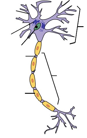
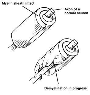
The data

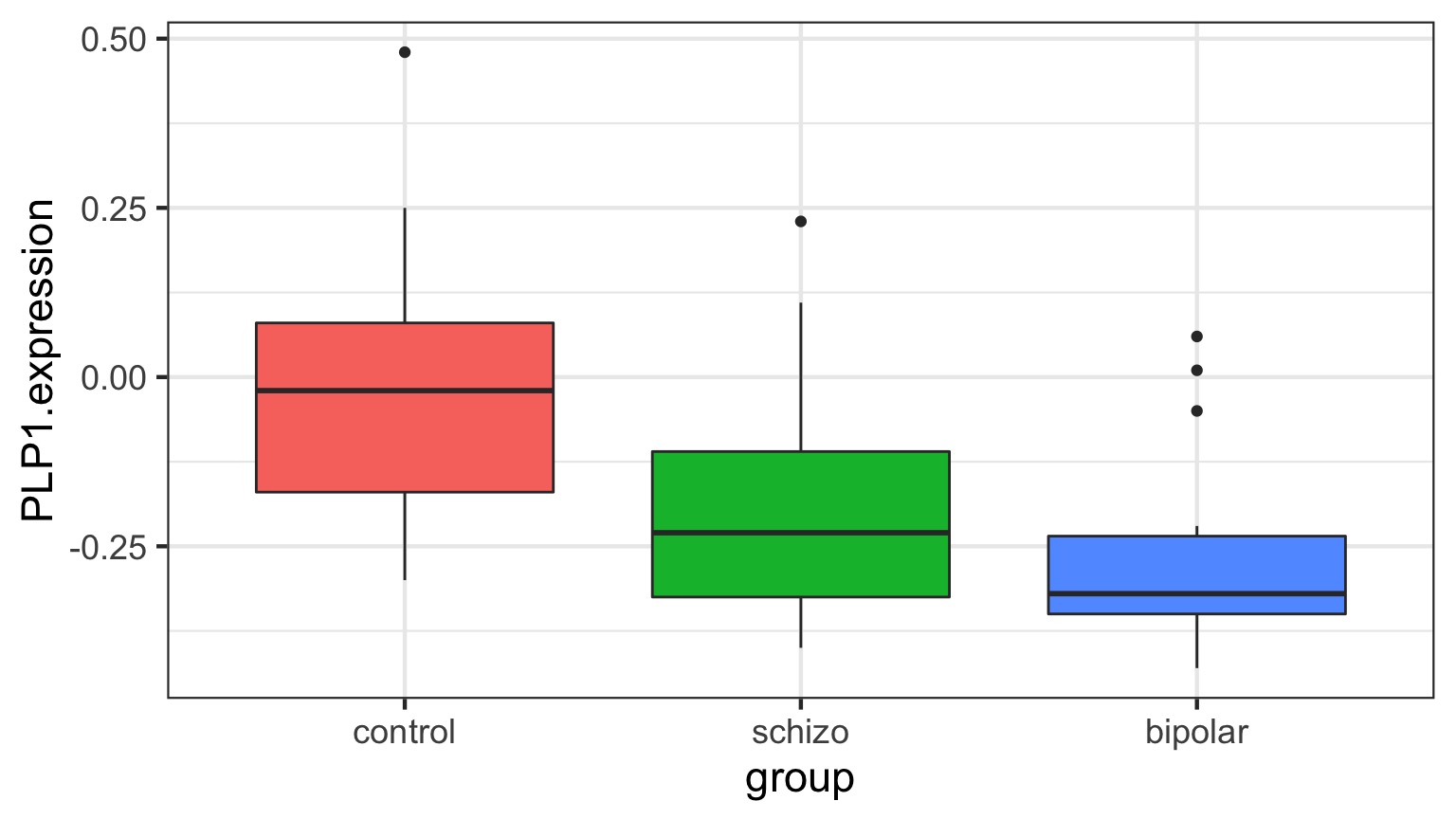
Comparison of Means

Means Model

\[\large y_{ij} = \alpha_{i} + \epsilon_{ij}, \qquad \epsilon_{ij} \sim N(0, \sigma^{2} )\]

Different mean for each group

Focus is on specificity of a categorical predictor

Questions we could ask

Does your model explain variation in the data?
Are your coefficients different from 0?
How much variation is retained by the model?
How confident can you be in model predictions?
Are groups different from each other

Questions we could ask

Does your model explain variation in the data?
Are your coefficients different from 0?
How much variation is retained by the model?
How confident can you be in model predictions?
Are groups different from each other

Testing the Model

Ho = The model predicts no variation in the data.

Ha = The model predicts variation in the data.

F-Tests

F = Mean Square Variability Explained by Model / Mean Square Error

DF for Numerator = k-1
DF for Denominator = n-k
k = number of groups, n = sample size

ANOVA

	Df	Sum Sq	Mean Sq	F value	Pr(>F)
group	2	0.5402533	0.2701267	7.823136	0.0012943
Residuals	42	1.4502267	0.0345292	NA	NA

Fitting an ANOVA model with Likelihood

brain_lik <- glm(PLP1.expression ~ group,
                 family=gaussian(),
                 data = brainGene)

\(\chi^2\) LR Test and ANOVA

	LR Chisq	Df	Pr(>Chisq)
group	15.64627	2	4e-04

This asks how much does the deviance change when we remove a suite of predictors from the model?

BANOVA

brain_brm <- brm(PLP1.expression ~ group, 
                 family = gaussian(link = "identity"),
                 data=brainGene,
                 file = "brain_brm.Rds")

BANOVA: Compare the relative magnitudes of variability due to Treatments

term	estimate	std.error	conf.low	conf.high
SD from Groups	0.1396133	0.0340588	0.0740639	0.2094102
SD from Residuals	0.1860021	0.0046805	0.1815504	0.1957638

Or via Percentages:

term	estimate	std.error	conf.low	conf.high
SD from Groups	43.09062	6.148865	29.89045	52.81145
SD from Residuals	56.90938	6.148865	47.18855	70.10955

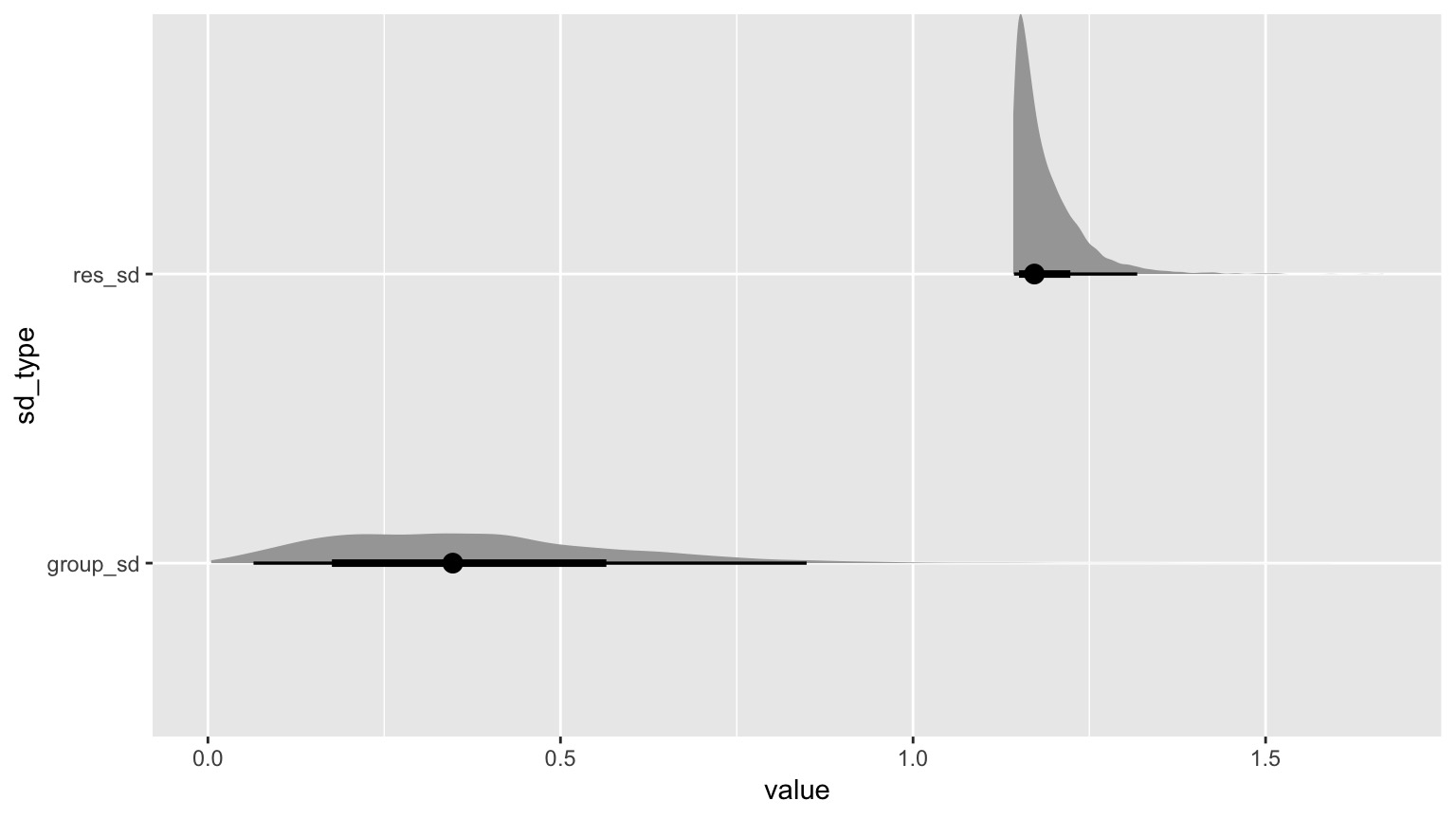
What if Treatment is relatively unimportant?

term	estimate	std.error	conf.low	conf.high
group_sd	0.3742119	0.2061628	0.0291503	0.7560807
res_sd	1.1878815	0.0494847	1.1421252	1.2808218

term	estimate	std.error	conf.low	conf.high
group_sd	22.86571	9.015793	4.387725	38.10253
res_sd	77.13429	9.015793	61.897473	95.61228

What if Treatment is relatively unimportant?

Questions we could ask

Does your model explain variation in the data?
Are your coefficients different from 0?
How much variation is retained by the model?
How confident can you be in model predictions?
Are groups different from each other

Questions we could ask

Does your model explain variation in the data?
Are your coefficients different from 0?
How much variation is retained by the model?
How confident can you be in model predictions?
Are groups different from each other

Outline

https://etherpad.wikimedia.org/p/607-anova

What can we ask of ANOVA?
Looking at treatment means
Tests of differences of means

ANOVA, F, and T-Tests

F-Tests	T-Tests
Tests if data generating process different than error	Tests if parameter is different from 0

Essentially comparing a variation explained by a model with versus without a data generating process included.

The Coefficients

	Estimate	Std. Error	t value	Pr(>\|t\|)
(Intercept)	-0.0040000	0.0479786	-0.0833705	0.9339531
groupschizo	-0.1913333	0.0678520	-2.8198628	0.0073015
groupbipolar	-0.2586667	0.0678520	-3.8122186	0.0004442

Treatment contrasts - set one group as a baseline
Useful with a control

Default “Treatment” Contrasts

        schizo bipolar
control      0       0
schizo       1       0
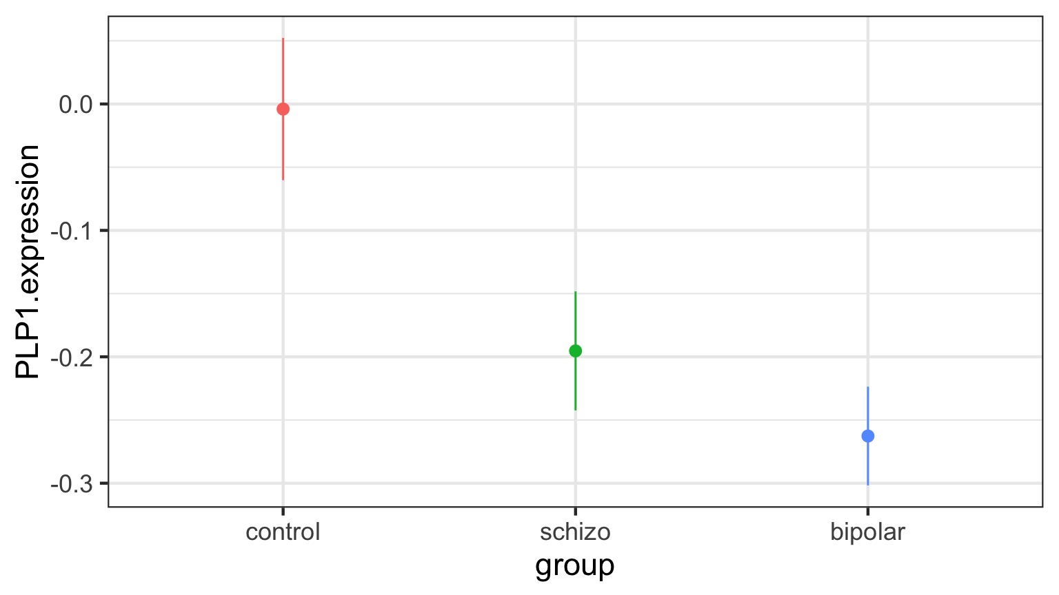
bipolar      0       1

Actual Group Means Compared to 0

contrast	estimate	SE	df	t.ratio	p.value
control effect	0.1500000	0.0391744	42	3.829034	0.0012669
schizo effect	-0.0413333	0.0391744	42	-1.055112	0.2974062
bipolar effect	-0.1086667	0.0391744	42	-2.773922	0.0123422

But which groups are different from each other?

Many T-tests….mutiple comparisons!

Outline

https://etherpad.wikimedia.org/p/607-anova

What can we ask of ANOVA?
Looking at treatment means
Tests of differences of means

The Problem of Multiple Comparisons

Solutions to Multiple Comparisons and Family-wise Error Rate?

Ignore it - a test is a test
- a priori contrasts
- Least Squares Difference test
Lower your \(\alpha\) given m = # of comparisons
- Bonferroni \(\alpha/m\)
- False Discovery Rate \(k\alpha/m\) where k is rank of test
Other multiple comparinson correction
- Tukey’s Honestly Significant Difference

ANOVA is an Omnibus Test

Remember your Null:
\[H_{0} = \mu_{1} = \mu{2} = \mu{3} = ...\]

This had nothing to do with specific comparisons of means.

A priori contrasts

Specific sets of a priori null hypotheses: \[\mu_{1} = \mu{2}\]
\[\mu_{1} = \mu{3} = ...\]

Use t-tests.

A priori contrasts

lm model parameter contrast

  Contrast   S.E.  Lower Upper    t df Pr(>|t|)
1    0.191 0.0679 0.0544 0.328 2.82 42   0.0073

A priori contrasts

lm model parameter contrast

                   Contrast   S.E.  Lower Upper    t df Pr(>|t|)
Control v. Schizo     0.191 0.0679 0.0544 0.328 2.82 42   0.0073
Control v. Bipolar    0.259 0.0679 0.1217 0.396 3.81 42   0.0004

Note: can only do k-1 before thinking about FWER, as each takes 1df

Orthogonal A priori contrasts

Sometimes you want to test very specific hypotheses about the structure of your groups

                     control schizo bipolar
Control v. Disorders       1   -0.5    -0.5
Bipolar v. Schizo          0    1.0    -1.0

Note: can only do k-1, as each takes 1df

Orthogonal A priori contrasts with Grouping


     Simultaneous Tests for General Linear Hypotheses

Fit: lm(formula = PLP1.expression ~ group, data = brainGene)

Linear Hypotheses:
                          Estimate Std. Error t value Pr(>|t|)  
Control v. Disorders == 0   0.2210     0.1018    2.17     0.07 .
Bipolar v. Schizo == 0      0.0673     0.0679    0.99     0.54  
---
Signif. codes:  0 '***' 0.001 '**' 0.01 '*' 0.05 '.' 0.1 ' ' 1
(Adjusted p values reported -- single-step method)

Post hoc contrasts

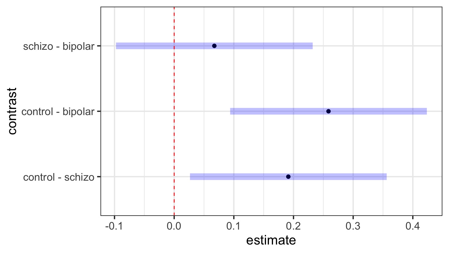
I want to test all possible comparisons!

No Correction: Least Square Differences

contrast	estimate	SE	df	t.ratio	p.value
control - schizo	0.191	0.068	42	2.820	0.007
control - bipolar	0.259	0.068	42	3.812	0.000
schizo - bipolar	0.067	0.068	42	0.992	0.327

P-Value Adjustments

Bonferroni : \(\alpha_{adj} = \frac{\alpha}{m}\) where m = # of tests
- VERY conservative

False Discovery Rate: \(\alpha_{adj} = \frac{k\alpha}{m}\)
- Order your p values from smallest to largest, rank = k,
- Adjusts for small v. large p values
- Less conservative

Other Methods: Sidak, Dunn, Holm, etc.
We’re very focused on p here!

Bonferroni Corrections

contrast	estimate	SE	df	t.ratio	p.value
control - schizo	0.191	0.068	42	2.820	0.022
control - bipolar	0.259	0.068	42	3.812	0.001
schizo - bipolar	0.067	0.068	42	0.992	0.980

p = m * p

FDR

contrast	estimate	SE	df	t.ratio	p.value
control - schizo	0.191	0.068	42	2.820	0.011
control - bipolar	0.259	0.068	42	3.812	0.001
schizo - bipolar	0.067	0.068	42	0.992	0.327

p = \(\frac{m}{k}\) * p

Other Methods Use Critical Values

Tukey’s Honestly Significant Difference
Dunnet’s Test for Comparison to Controls
Ryan’s Q (sliding range)
etc…

Tukey’s Honestly Significant Difference

contrast	estimate	SE	df	t.ratio	p.value
control - schizo	0.191	0.068	42	2.820	0.020
control - bipolar	0.259	0.068	42	3.812	0.001
schizo - bipolar	0.067	0.068	42	0.992	0.586

Visualizing Comparisons (Tukey)

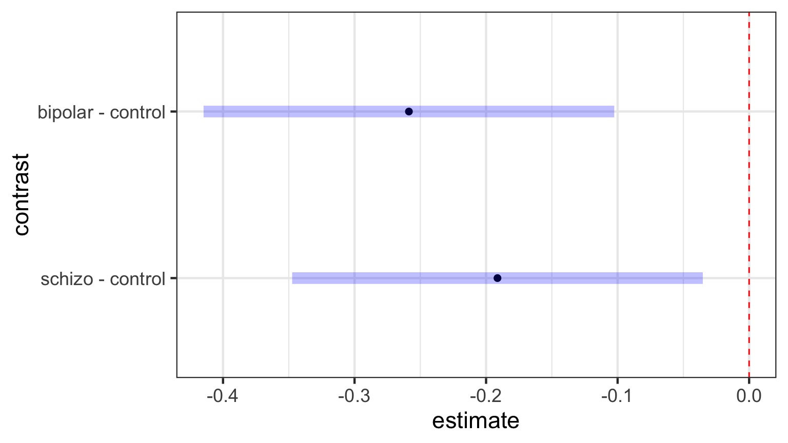
Dunnett’s Comparison to Controls

contrast	estimate	SE	df	t.ratio	p.value
schizo - control	-0.191	0.068	42	-2.82	0.014
bipolar - control	-0.259	0.068	42	-3.81	0.001

Likelihood and Posthocs

group	emmean	SE	df	asymp.LCL	asymp.UCL
control	-0.004	0.048	Inf	-0.098	0.090
schizo	-0.195	0.048	Inf	-0.289	-0.101
bipolar	-0.263	0.048	Inf	-0.357	-0.169

Posthocs Use Z-tests

contrast	estimate	SE	df	z.ratio	p.value
control - schizo	0.191	0.068	Inf	2.820	0.013
control - bipolar	0.259	0.068	Inf	3.812	0.000
schizo - bipolar	0.067	0.068	Inf	0.992	0.582

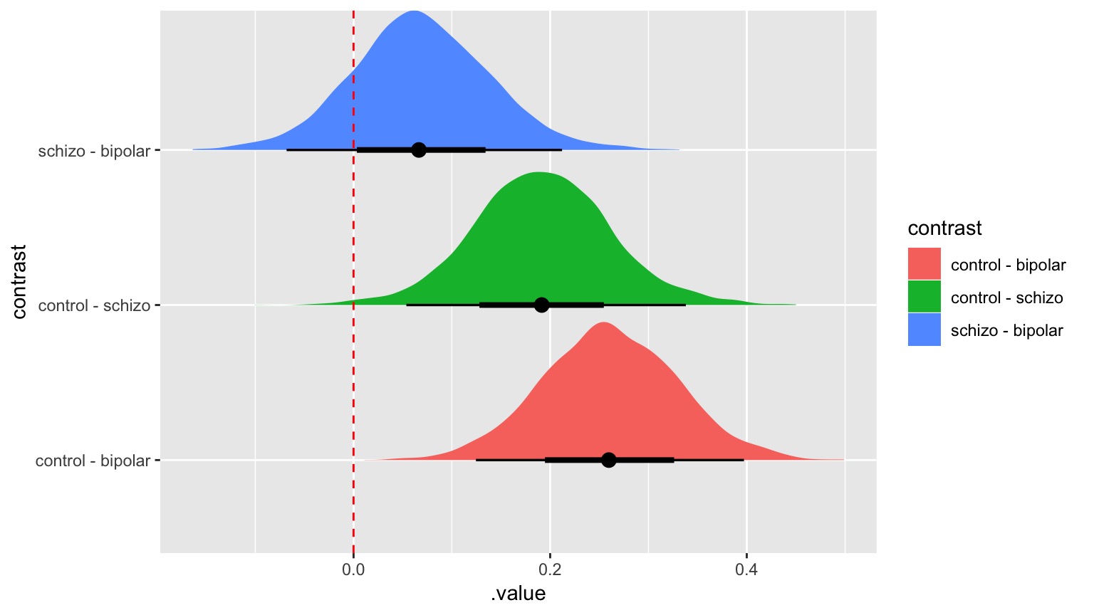
Bayes-Style!

group	emmean	lower.HPD	upper.HPD
control	-0.003	-0.100	0.091
schizo	-0.195	-0.288	-0.095
bipolar	-0.263	-0.362	-0.163

Bayes-Style!

Final Notes of Caution

Often you DO have a priori contrasts in mind
If you reject Ho with ANOVA, differences between groups exist
Consider Type I v. Type II error before correcting