Bayesian Statistics: an introduction
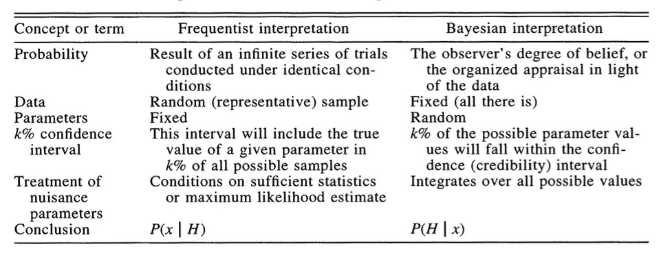
Bayesian Inference
Estimate probability of a parameter
State degree of believe in specific parameter values
Evaluate probability of hypothesis given the data
Incorporate prior knowledge
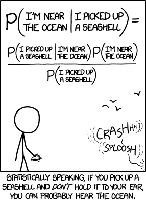
Bayes Theorem
We know…\[\huge p(a\ and\ b) = p(a)p(b|a)\]
Bayes Theorem
And Also…\[\huge p(a\ and\ b) = p(b)p(a|b)\]
Bayes Theorem
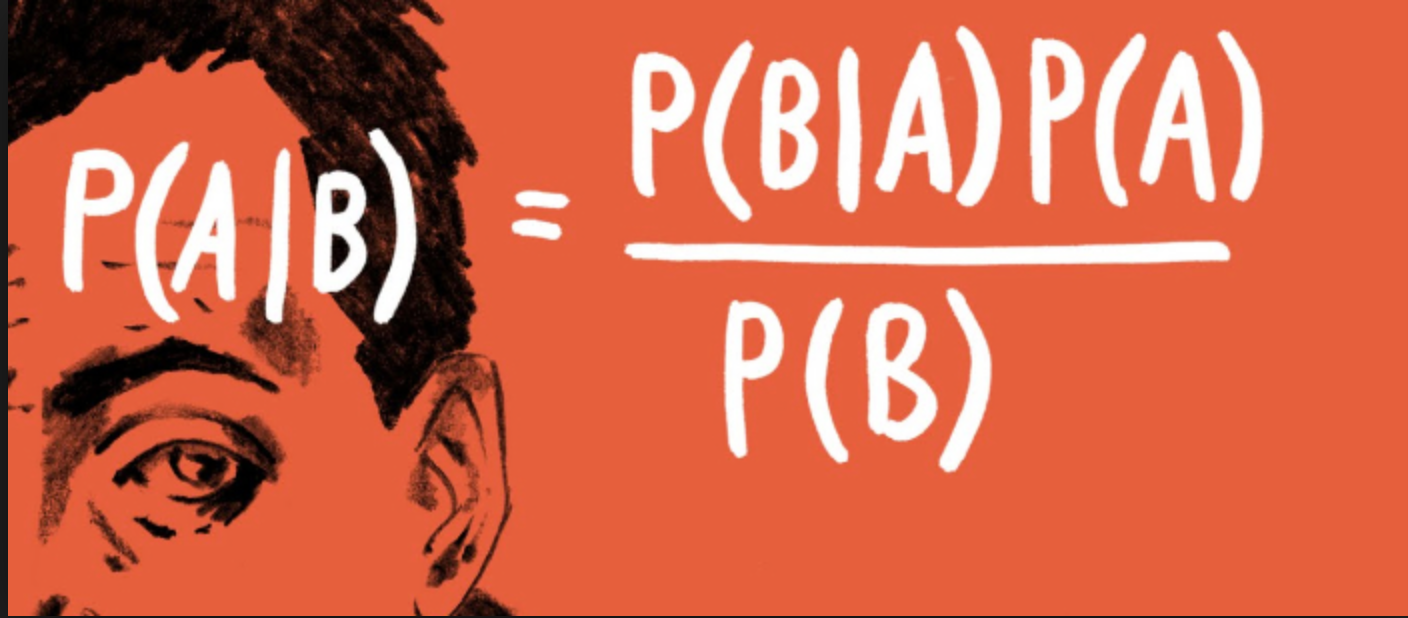
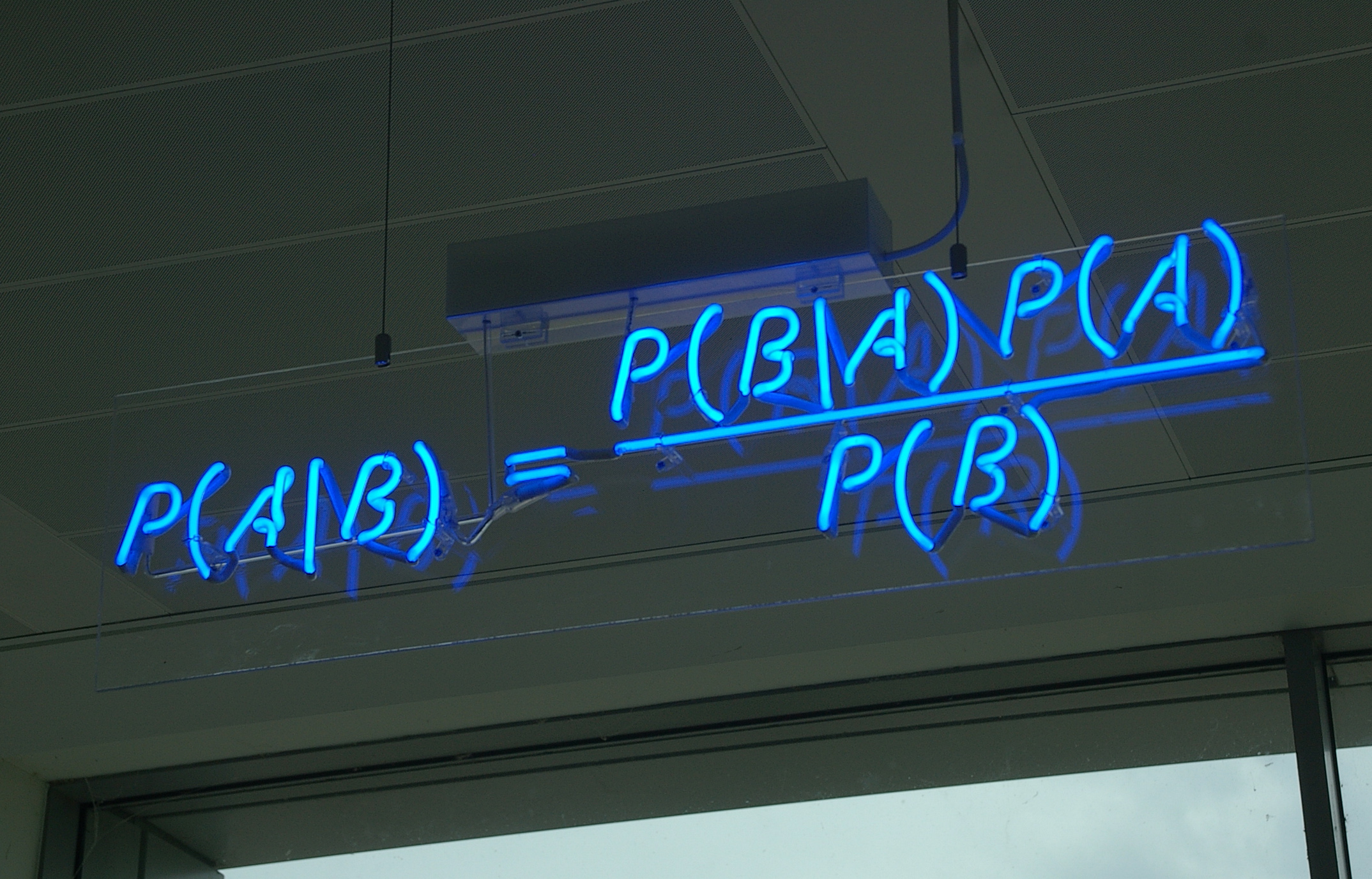
And thus…
\[\huge p(a|b) = \frac{p(b|a)p(a)}{p(b)} \]
What is a posterior distribution?
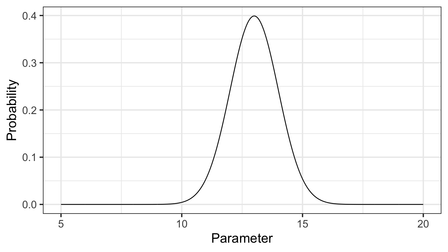
What is a posterior distribution?
The probability that the parameter is 13 is 0.4
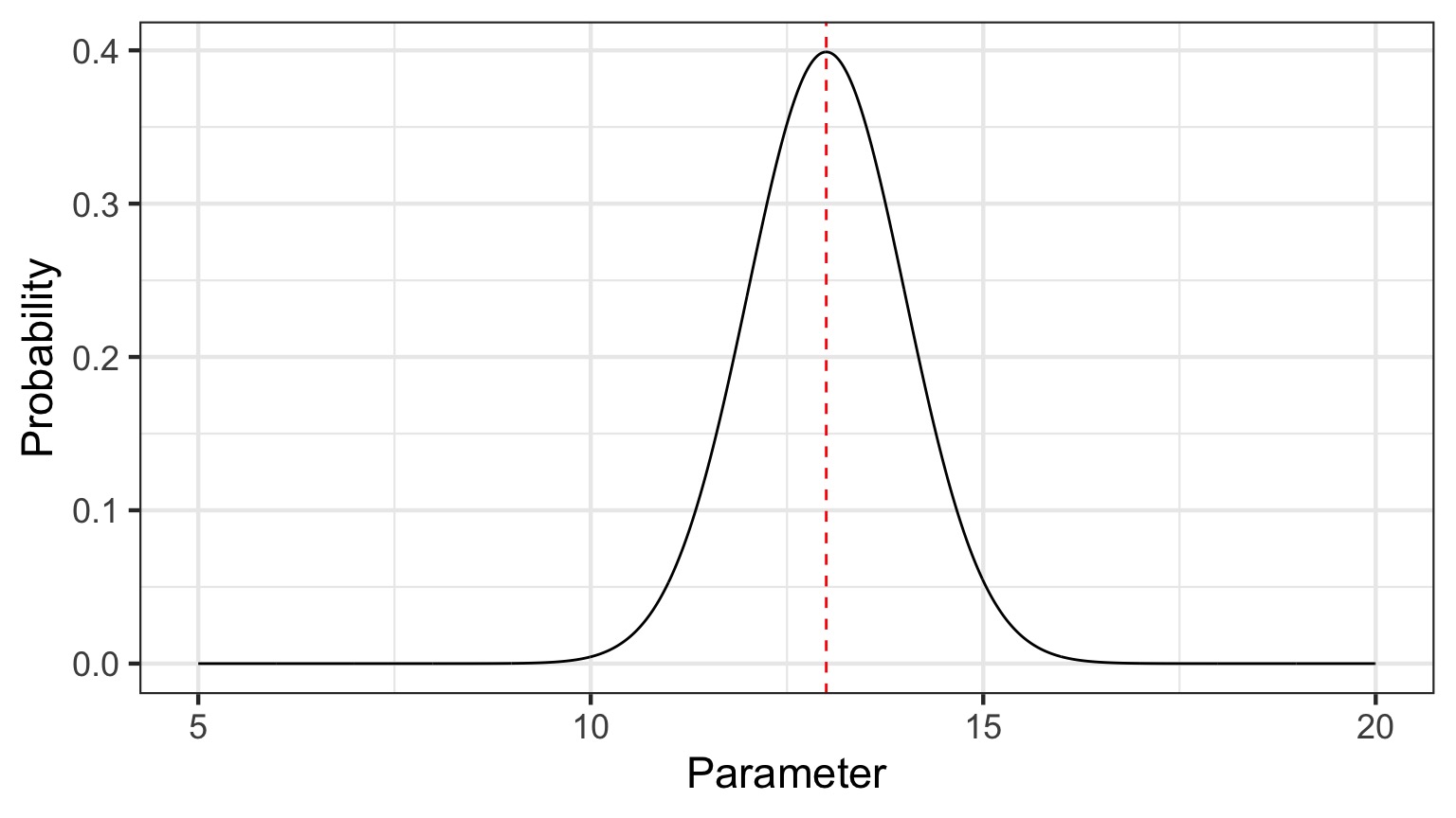
What is a posterior distribution?
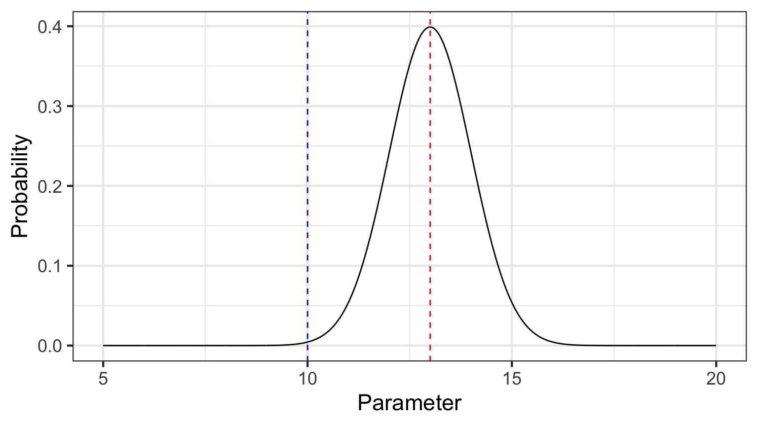
The probability that the parameter is 13 is 0.4
The probability that the parameter is 10 is 0.044
What is a posterior distribution?
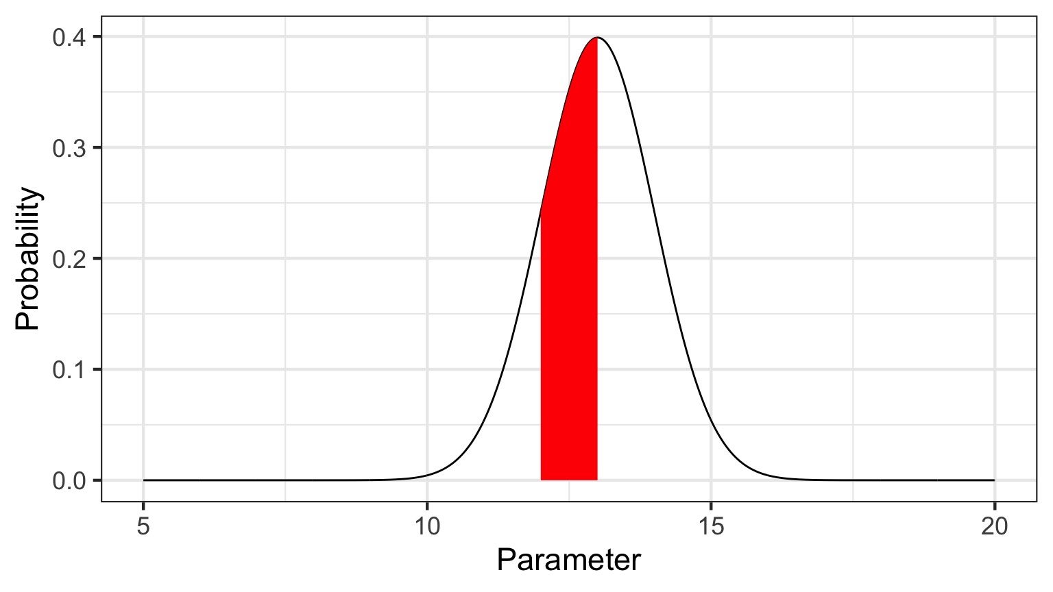
Probability that parameter is between 12 and 13 = 0.3445473
Bayesian Credible Interval
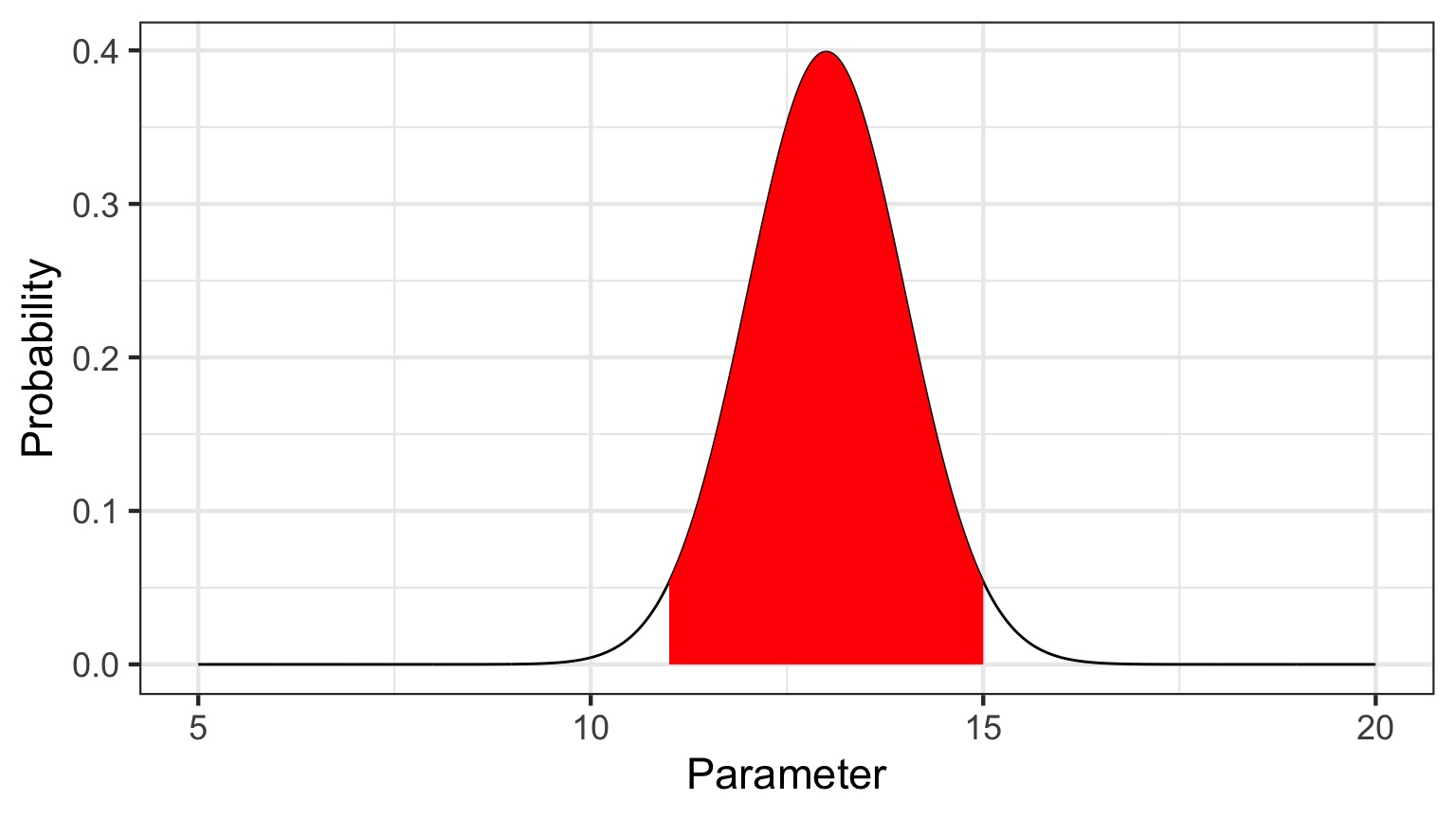
Area that contains 95% of the probability mass of the posterior distribution
Degree of believe in a result
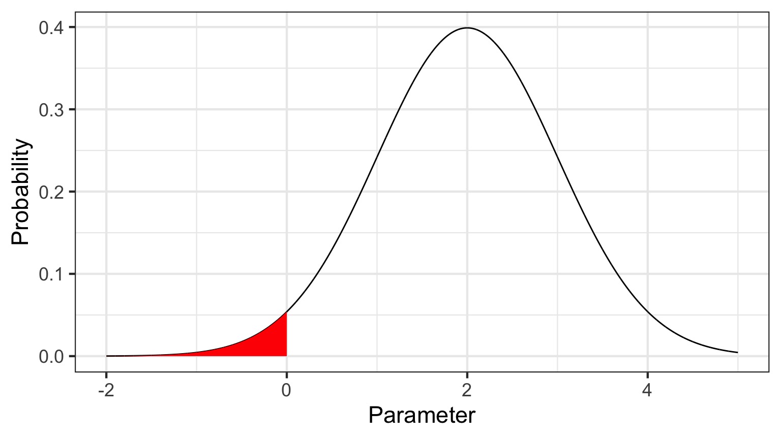
You can discuss the probability that your parameter is opposite in sign to its posterior modal estimate. This yields a degree of belief that you at least have the sign correct (i.e., belief in observing a non-zero value)
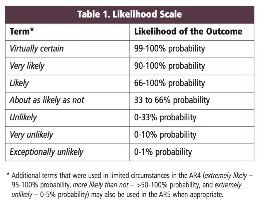
Talking about Uncertainty the IPCC Way
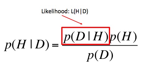
Hello Again, Likelihood
Prior Probability
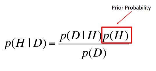
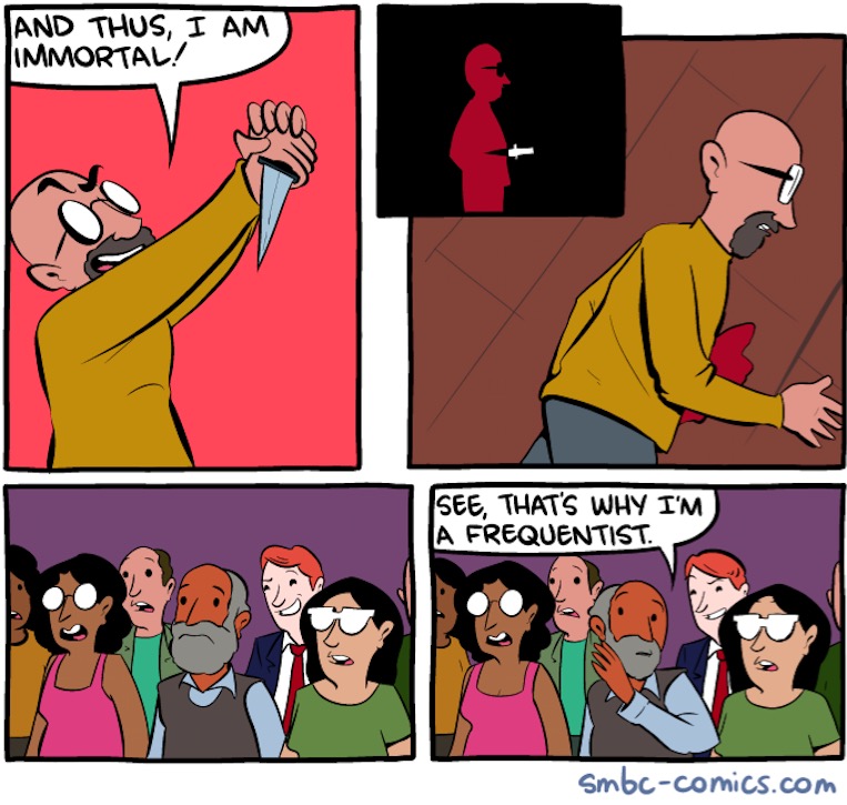
This is why Bayes is different from Likelihood!
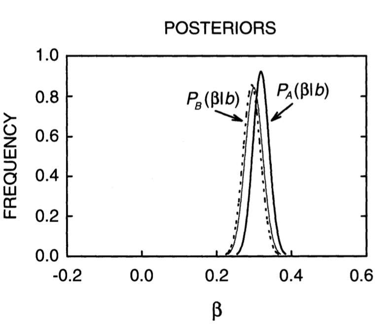
The Influence of Priors

The Influence of Priors
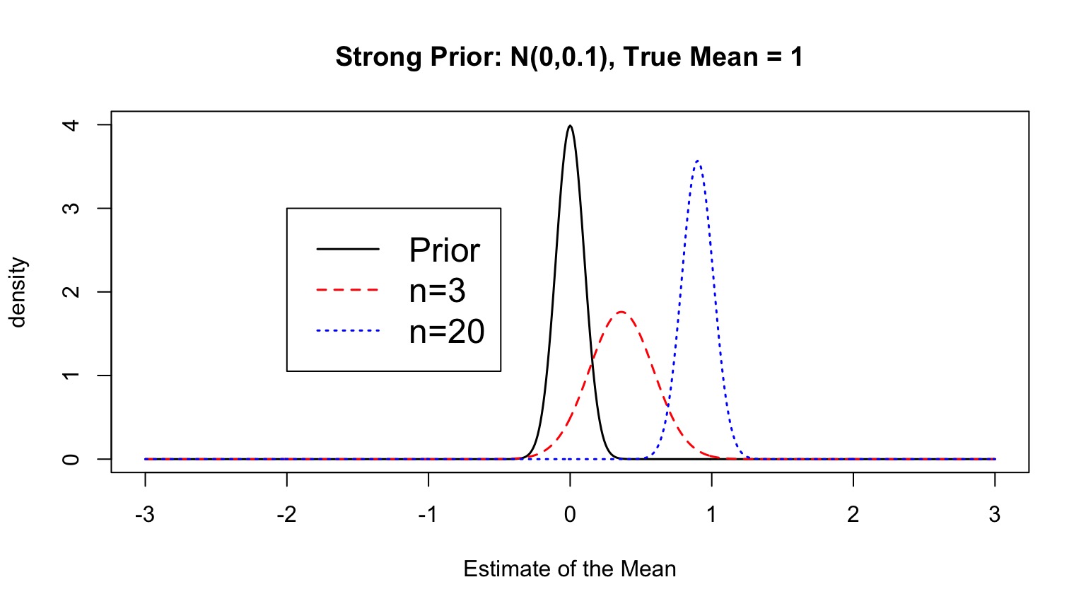
Priors and Sample Size
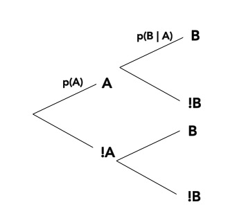
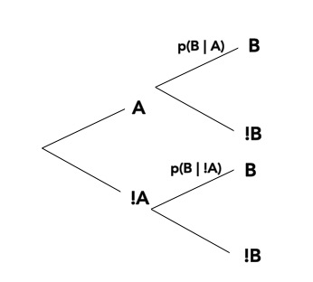
p(data) is just a big summation/integral
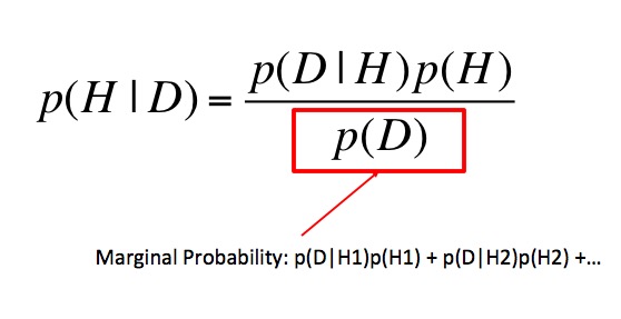
Denominator: The Marginal Distribution
Essentially, all alternate hypotheses
Denominator - marginal distribution - becomes an integral of likelihoods if \(B\) is continuous - i.e. fitting a particular parameter value. It normalizes the equation to be between 0 and 1.


Bayes Theorem in Action
Where have we gone?
Ellison 1996