Fitting Models with Likelihood!

Outline

1. Review of Likelihood
   
   
2. Comparing Models with Likelihood
   
   
3. Linear Regression with Likelihood
   

Deriving Truth from Data

• Frequentist Inference: Correct conclusion drawn from repeated experiments
  • Uses p-values and CIs as inferential engine
    
    
• Likelihoodist Inference: Evaluate the weight of evidence for different hypotheses
  • Derivative of frequentist mode of thinking
    
  • Uses model comparison (sometimes with p-values…)
    
    
• Bayesian Inference: Probability of belief that is constantly updated
  • Uses explicit statements of probability and degree of belief for inferences

Likelihood: how well data support a given hypothesis.

Note: Each and every parameter choice IS a hypothesis

Likelihood Defined

\[\Large L(H | D) = p(D | H)\]

Where the D is the data and H is the hypothesis (model) including a both a data generating process with some choice of parameters (aften called \(\theta\)). The error generating process is inherent in the choice of probability distribution used for calculation.

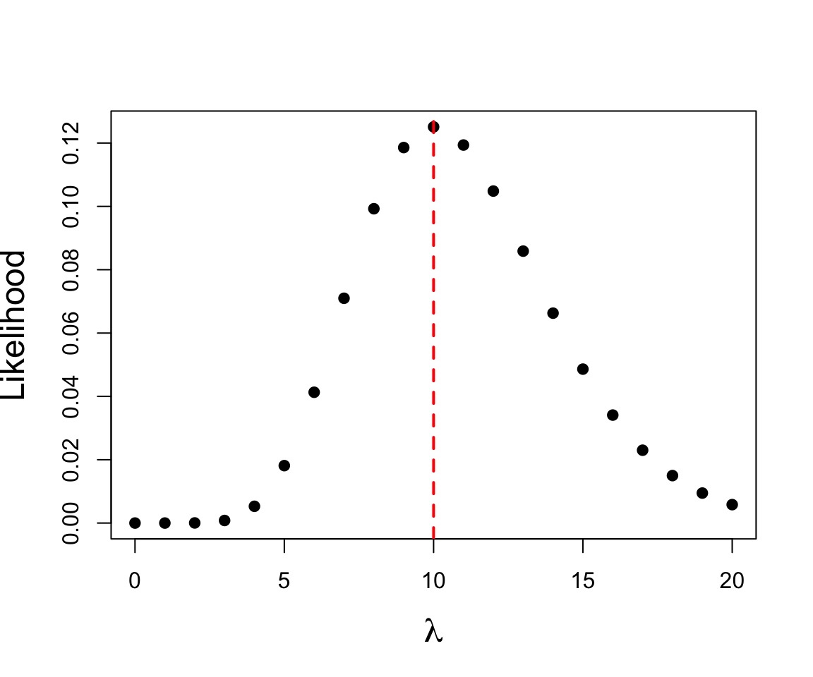
Example of Maximum Likelihood Fit

Let’s say we have counted 10 individuals in a plot. Given that the population is Poisson distributed, what is the value of \(\lambda\)?

Likelihood Function

\[\Large p(x) = \frac{\lambda^{x}e^{-\lambda}}{x!}\]

• This is a Likelihood Function for one sample
  
  • It is the Poisson Probability Density function
    
    
• \(Dpois = \frac{\lambda^{x}e^{-\lambda}}{x!}\)
  

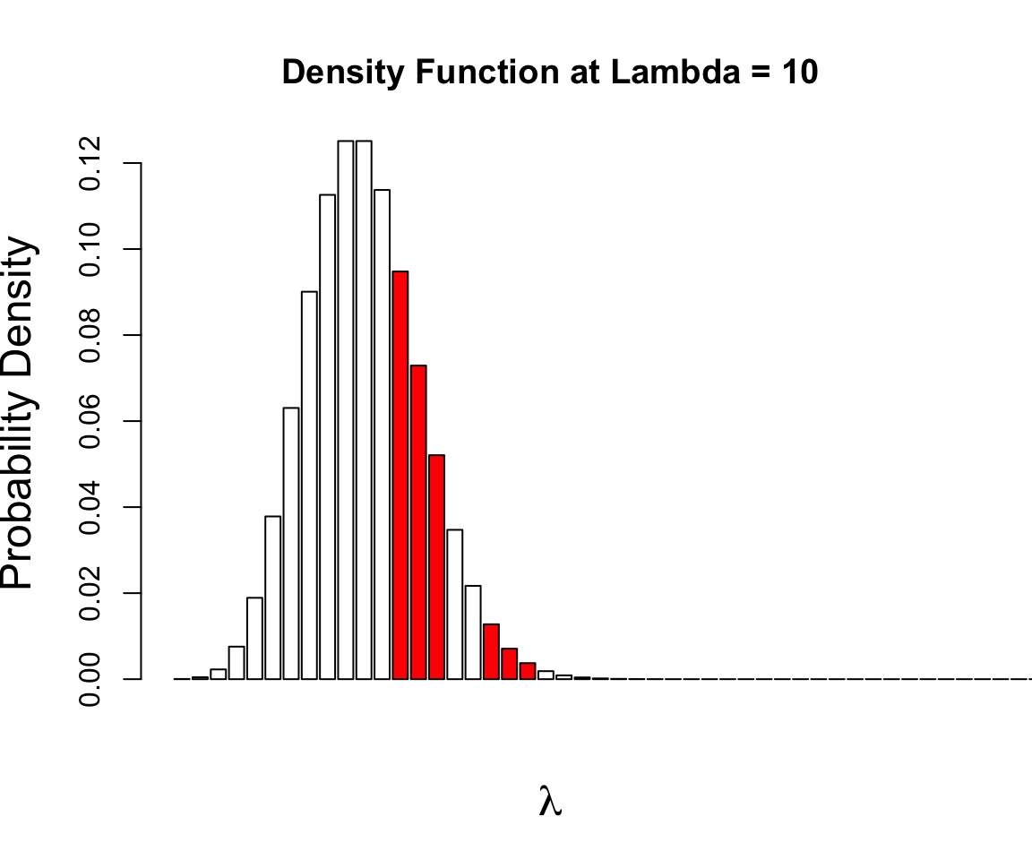
What is the probability of the data given the parameter?

Outline

1. Review of Likelihood
   
   
2. Comparing Models with Likelihood
   
   
3. Linear Regression with Likelihood
   

Can Compare p(data | H) for alternate Parameter Values

Compare \(p(D|\theta_{1})\) versus \(p(D|\theta_{2})\)

Likelihood Ratios

\[\LARGE G = \frac{L(H_1 | D)}{L(H_2 | D)}\]

• G is the ratio of Maximum Likelihoods from each model
  
  
• Used to compare goodness of fit of different models/hypotheses
  
  
• Most often, \(\theta\) = MLE versus \(\theta\) = 0
  
  
• \(-2 log(G)\) is \(\chi^2\) distributed

Likelihood Ratio Test

• A new test statistic: \(D = -2 log(G)\)
   
• \(= 2 [Log(L(H_2 | D)) - Log(L(H_1 | D))]\)
  
  
• It’s \(\chi^2\) distributed!
  - DF = Difference in # of Parameters
  
  
• If \(H_1\) is the Null Model, we have support for our alternate model

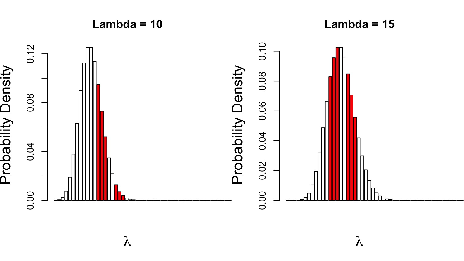
Likelihood Ratio at Work

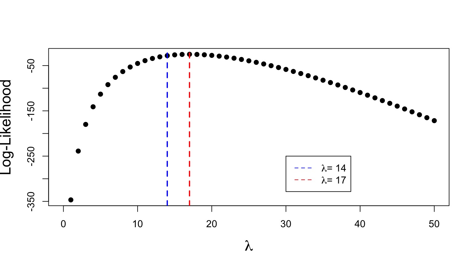
\[G = \frac{L(\lambda = 14 | D)}{L(\lambda = 17 | D)}\]
=0.0494634

Likelihood Ratio Test at Work

\[D = 2 [Log(L(\lambda = 14 | D)) - Log(L(\lambda = 17 | D))]\] =6.0130449 with 1DF
p =0.01

Outline

1. Review of Likelihood
   
   
2. Comparing Models with Likelihood
   
   
3. Linear Regression with Likelihood
   

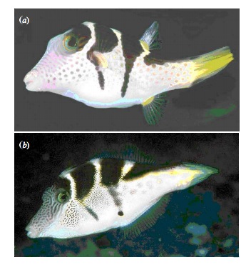
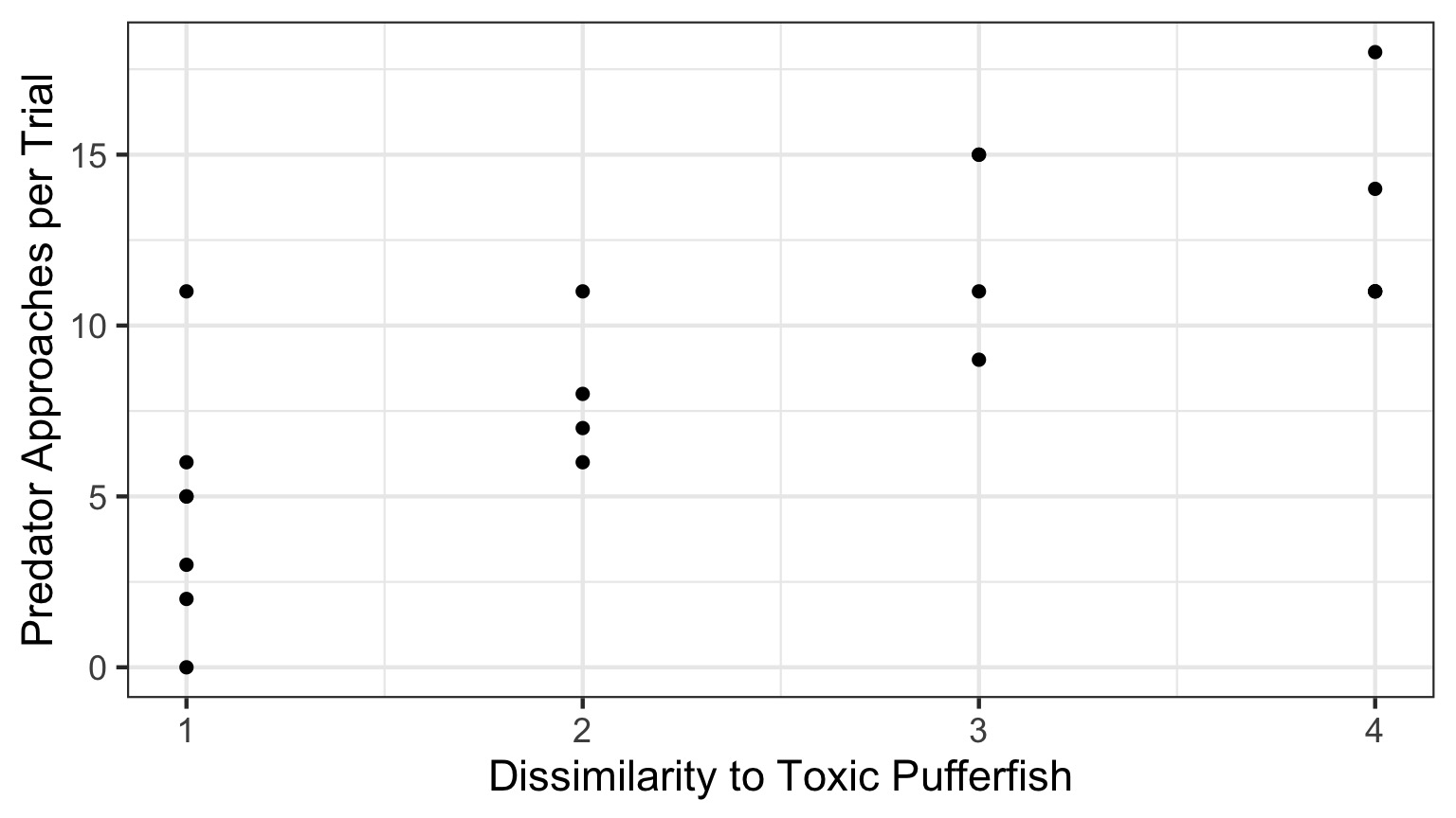
Putting Likelihood Into Practice with Pufferfish

Does Resembling a Pufferfish Reduce Predator Visits?

The Steps of Statistical Modeling

1. What is your question?
2. What model of the world matches your question?
3. Build a test
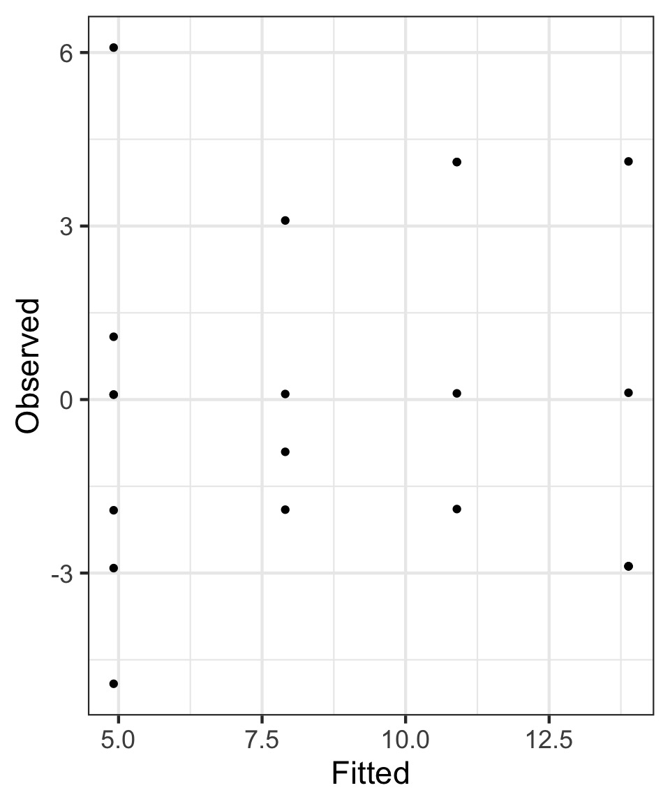
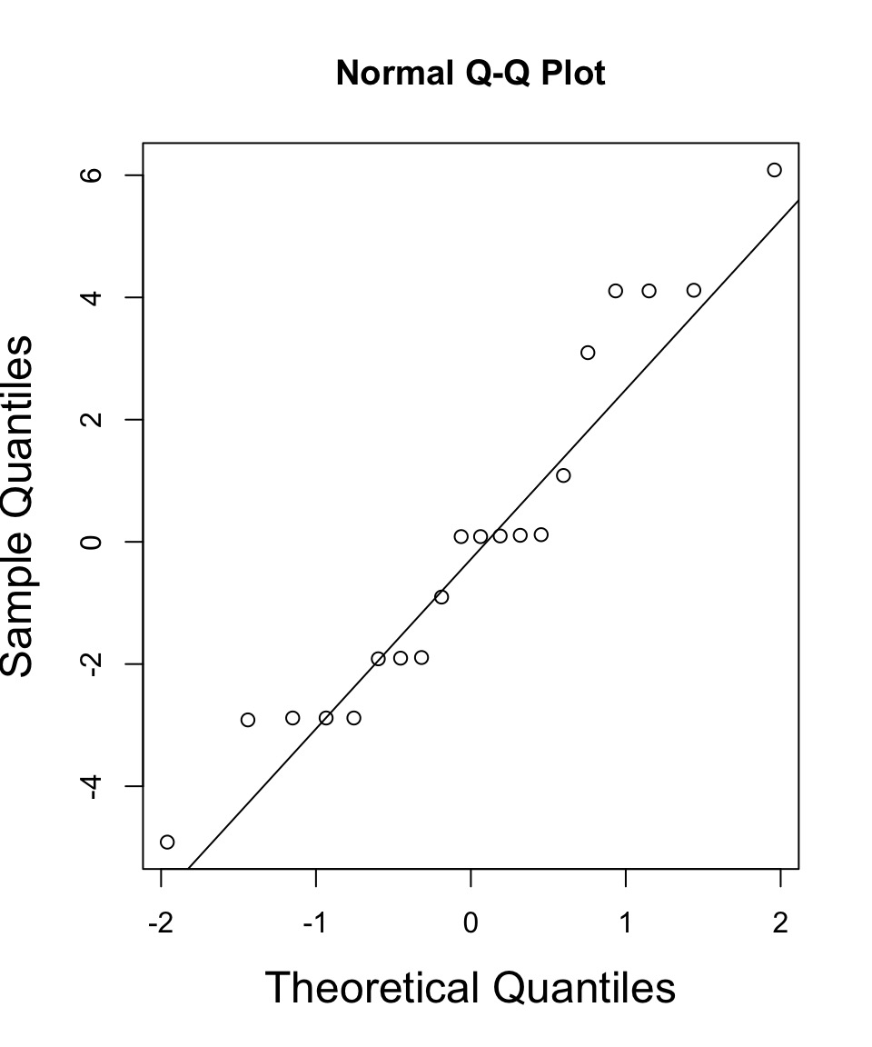
4. Evaluate test assumptions
5. Evaluate test results
6. Visualize

The World of Pufferfish

Data Generating Process:

Error Generating Process:

Quantiative Model of Process Using Likelihood

Likelihood:
\(Visits_i \sim \mathcal{N}(\hat{Visits_i}, \sigma)\)



Data Generating Process:
\(\hat{Visits_i} = \beta_{0} + \beta_{1} Resemblance_i\)

Likelihood Function for Linear Regression

Likelihood Function for Linear Regression

\[L(\theta | Data) = \prod_{i=1}^n \mathcal{N}(Visits_i\; |\; \beta_{0} + \beta_{1} Resemblance_i, \sigma)\]

where \(\beta_{0}, \beta_{1}, \sigma\) are elements of \(\theta\)

Quantiative Model of Process Using Likelihood

Likelihood:
\(Visits_i \sim \mathcal{N}(\hat{Visits_i}, \sigma)\)



Data Generating Process:
\(\hat{Visits_i} = \beta_{0} + \beta_{1} Resemblance_i\)

Fit Your Model!

puffer_glm <- glm(predators ~ resemblance, 
                  data = puffer,
                  family = gaussian(link = "identity"))

The Same Diagnostics

But - What do the Likelihood Profiles Look Like?

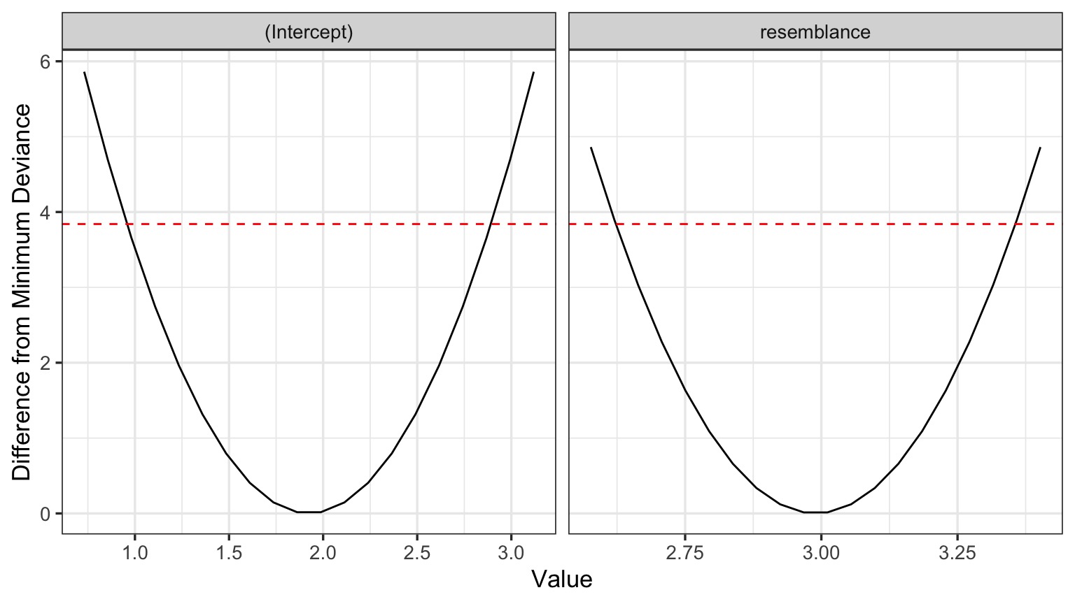
Are these nice symmetric slices?

Sometimes Easier to See with a Straight Line

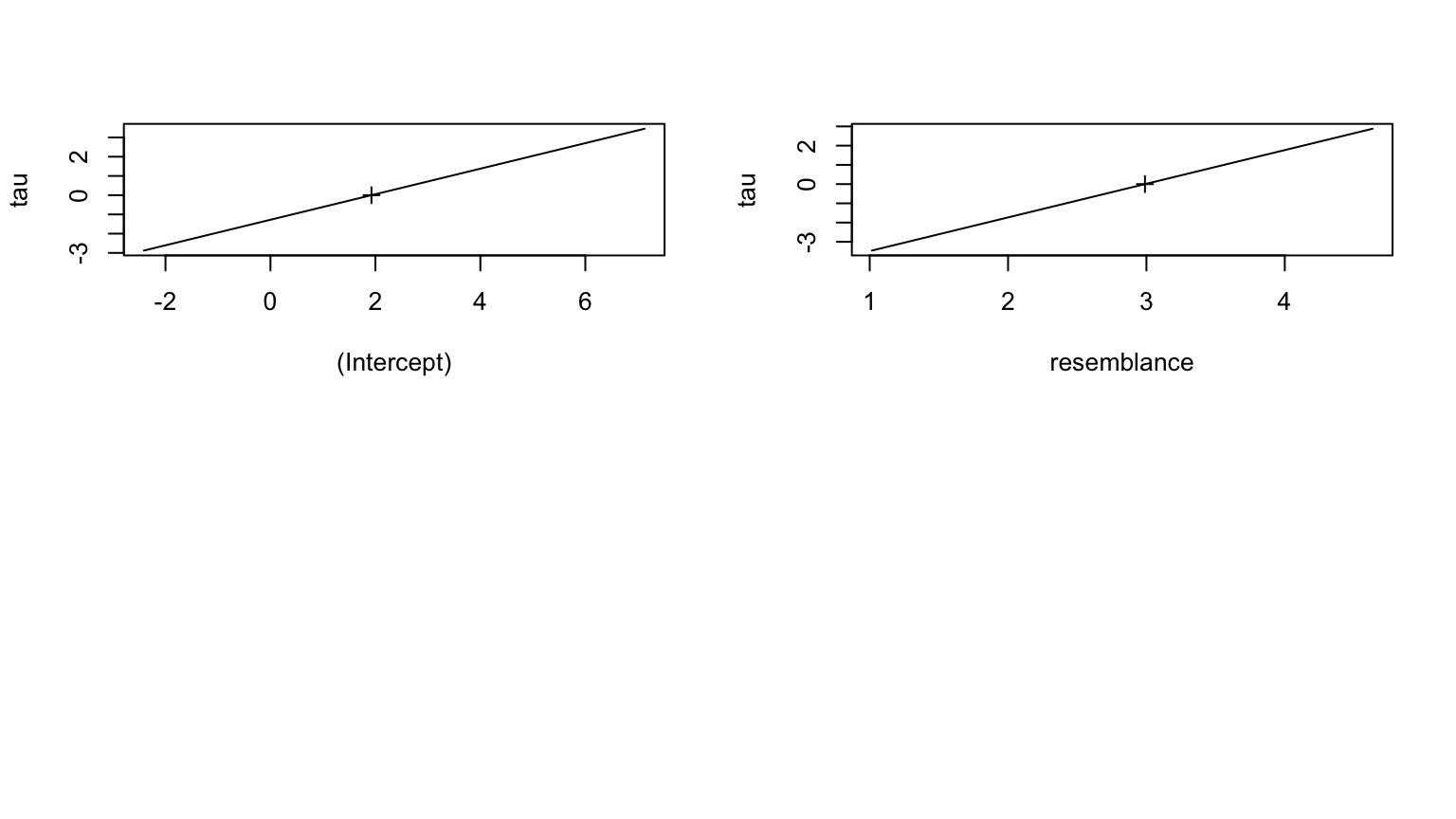
tau = signed sqrt of difference from deviance

Evaluate Coefficients

Test Statistic is a Wald Z-Test Assuming a well behaved quadratic Confidence Interval

Confidence Intervals

To test the model, need an alternate hypothesis

Put it to the Likelihood Ratio Test!

Analysis of Deviance Table

Model 1: predators ~ 1
Model 2: predators ~ resemblance
  Resid. Df Resid. Dev Df Deviance  Pr(>Chi)    
1        19     422.95                          
2        18     167.80  1   255.15 1.679e-07 ***
---
Signif. codes:  0 '***' 0.001 '**' 0.01 '*' 0.05 '.' 0.1 ' ' 1

Compare to Linear Regression

Compare to Linear Regression: F and Chisq