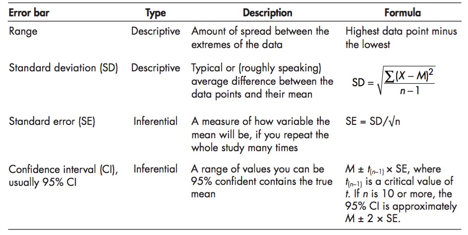
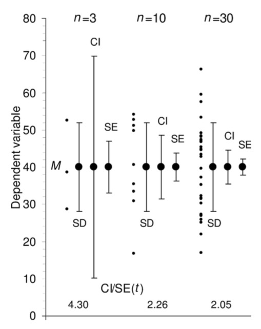
Sampling Estimate, Precision, and Simulation

class: middle, center

# Sampling Distributions

![](./images/04/meanception.jpg)

---
# Last Time: Sample Versus Population

---

# Sample Properties: **Mean**

`$$\bar{x} = \frac{ \displaystyle \sum_{i=1}^{n}{x_{i}} }{n}$$`

`$\large \bar{x}$` - The average value of a sample  
`$x_{i}$` - The value of a measurement for a single individual   
n - The number of individuals in a sample  
&nbsp;  
`$\mu$` - The average value of a population  
(Greek = population, Latin = Sample)

---
class: center, middle

# Our goal is to get samples representative of a population, and estimate population parameters. We assume a **distribution** of values to the population.

---
# Probability Distributions
<img src="04_sampling_dist_files/figure-html/normplot-1.png" style="display: block; margin: auto;" />

---

# Probability Distributions Come in Many Shapes

---

# Sample Versus Sampling Distributions

- A sampling distribution is the distribution of estimates of population parameters if we repeated our study an infinite number of times.

- For example, if we take a sample with n = 5 of plant heights, we might get a mean of 10.5cm. If we do it again, 8.6cm. Again, 11.3cm, etc....  
  
- Repeatedly sampling gives us a distribution, and a measure of how precise our ability to estimate a population parameter is

---

class:middle

.center[![:scale 95%](images/04/Accuracy-and-Precision.png)]

- Accuracy represents *is your estimate of a population parameter baised*. 
  
- Precision tells us the *variability in replicate measurements of a population parameter*

---
# A simple simulation

Let's say you sampled a population of corals and assessed Zooxanthelle concentration. You did this with n = 10, an then calculated the average concentration per coral.

---
# A simple simulation

Now do it again 10 more times

---
# What's the Distribution of Those Means?

---
# What About After 1000 repeated sample events with n = 10?

<img src="04_sampling_dist_files/figure-html/mean_100-1.png" style="display: block; margin: auto;" />
--

This is a **sampling distribution** and looks normal for the mean.

---
# Does Sample Size Matter?

This looks normal, with different SD?

---
class: center, middle
# **Central Limit Theorem** The distribution of means of a sufficiently large sample size will be approximately normal

https://istats.shinyapps.io/sampdist_cont/

https://istats.shinyapps.io/SampDist_discrete/

## This is true for many estimated parameters based on means

---
# So what about the SD of the Simulated Estimated Means?

---
class: center, middle
# The Standard Error
<br><br>
.large[
A standard error is the standard deviation of an estimated parameter if we were able to sample it repeatedly. It measures the precision of our estimate.
]

---
class: large

# So I always have to repeat my study to get a Standard Error?

## .center[**No**]

Many common estimates have formulae, e.g.:

`$$SE_{mean} = \frac{s}{\sqrt(n)}$$`

---

# Others Have Complex Formulae for a Single Sample, but Still Might be Easier to Get Via Simulation - e.g., Standard Deviation

```
     2.5%       33%       66%     97.5% 
 1.189182  4.462456  7.290618 12.960790 
```

---
class: large

# Standard Error as a Measure of Confidence
--

.center[.red[**Warning: this gets weird**]]

- We have calculated our SE from a **sample** - not the **population**

- Our estimate ± 1 SE tells us 2/3 of the *means* we could get by **resampling this sample**

- This is **not** 2/3 of the possible **true parameter values**

- BUT, if we *were* to sample the population many times, 2/3 of the time, the sample-based SE will contain the "true" value

---

# Confidence Intervals

.large[
- So, 1 SE = the 66% Confidence Interval

- ~2 SE = 95% Confidence Interval

- Best to view these as a measure of precision of your estimate

- And remember, if you were able to do the sampling again and again and again, some fraction of your intervals would *not* contain a true value
]
---

class: large, middle

# Let's see this in action

### .center[.middle[https://istats.shinyapps.io/ExploreCoverage/]]

---

# Frequentist Philosophy

.large[The ideal of drawing conclusions from data based on properties derived from theoretical resampling is fundamentally **frequentist** - i.e., assumes that we can derive truth by observing a result with some frequency in the long run.]

---
# SE, SD, CIs.... They are Different

![:scale 95%](images/04/cumming_table_2007.jpg)

.bottom[.small[.left[[Cumming et al. 2007 Table 1](http://byrneslab.net/classes/biol-607/readings/Cumming_2007_error.pdf)]]]

---
# SE (sample), CI (sample), and SD (population) visually

.center[![:scale 55%](images/04/cumming_comparison_2007.jpg)]

.bottom[.small[.left[[Cumming et al. 2007 Table 1](http://byrneslab.net/classes/biol-607/readings/Cumming_2007_error.pdf)]]]

---
# So what does this mean?

---
# 95% CI and Frequentist Logic

- Having 0 in your 95% CI means that, we you to repeat an analysis 100 times, 0 will be in 95 of the CIs of those trials.

- In the long run, you have a 95% chance of being wrong if you say that 0 is not a possible value.

- But..... why 95%? Why not 80% Why not 75%? 95% can be finicky!

- Further, there is no probability of being wrong about sign, just, in the long run, you'll often have a CI overlapping 0 given the design of your study

- A lot depends on how well you trust the precision of your estimate based on your study design