Samples and Populations

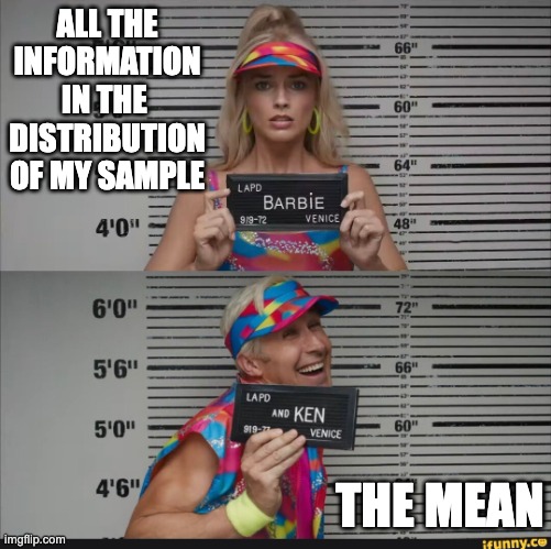
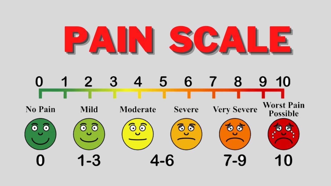
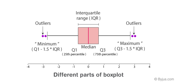
class: middle, center
background-position: center
background-size: cover

# Sample Distributions
<br>
![](images/03/barbie_sample_distribution_mean.jpg)

---
# Outline

1. What is a Good Sample?

2. Sample Distributions and Parameters

3. Non-parameteric Properties of Samples and Populations

---
class:center

# What is a population?

**Population** = All Individuals

---
class: center, middle
# Population
.pull-left[
<img src="03_sampling_lecture_x_files/figure-html/population-1.png" style="display: block; margin: auto;" />
]

.pull-right[
<img src="03_sampling_lecture_x_files/figure-html/normplot3-1.png" style="display: block; margin: auto;" />
]
---
class: center

# What is a sample?

--
A **sample** of individuals in a randomly distributed population.

---
class: center, middle
# Population
.pull-left[
<img src="03_sampling_lecture_x_files/figure-html/sampleSpread-1.png" style="display: block; margin: auto;" />
]

.pull-right[
<img src="03_sampling_lecture_x_files/figure-html/normplotsamp-1.png" style="display: block; margin: auto;" />
]

---
# Properties of a good sample

1. Validity  
    - Yes, this is a measure of what I am interested in

2. Reliability  
      - If I sample again, I'll get something similar

3. Representative
      - Sample reflects the population
      - Unbiased

---

# Validity: Is it measuring what I think it's measuring?

.center[![:scale 75%](./images/03/23andme_health_ancestry_kit.jpg)]

---

# Reliability: Is my sample/measure repeatable?

.center[![](./images/03/painscale.jpg)]

---

# Are You Representative? Or Biased from Unequal Representation
<img src="03_sampling_lecture_x_files/figure-html/spatialBias-1.png" style="display: block; margin: auto;" />
If you only chose individuals from the bottom, you would only get one range of sizes.

---
class: center, middle

## The key for most statistical models is that a replicates in a sample are i.i.d.  
  
  <br>
  
## Independent and Identically Distributed

---
# Exercise:
<br><br>
### 1. What is a population you sample?  
  <br><br>
  
### 2. How do you ensure validity, reliability, and representativeness of a sample from your population?

---
# Outline

1. What is a Good Sample?

2. .red[Sample Distributions and Parameters]

3. Non-parameteric Properties of Samples and Populations

---
# Taking a Descriptive
<img src="03_sampling_lecture_x_files/figure-html/sampleSpread-1.png" style="display: block; margin: auto;" />

<center>How big are individuals in this population?

---
# Our 'Sample'

---

# Visualizing Our Sample as Counts with 20 Bins

---

# Visualizing Our Sample as Frequencies

--
Frequency = % of Sample with that Value

---

# Visualizing Our Sample as Frequencies

Frequency = Probability of Drawing that Value from a Sample

---

# Visualizing Our Sample as Continuous Probability Densities

Probability Density = Relative likleihood of encountering a value. Sums to One.

---
class: center, middle

# Our goal is to get samples representative of a population, and estimate population parameters. We assume a **distribution** of values to the population from which we then estimate parameters. Makes it easier to describe nature!

---
# A Population versus Sample Distribution: Normal

---

# The Normal (Gaussian) Distribution

- Arises from some deterministic value and many small additive deviations. 
- Variability is additive over time.
- VERY common.

---
class: center

# Understanding Gaussian Distributions with a Galton Board (Quinqunx)

---

# We see this pattern everywhere - the Random or Drunkard's Walk aka Brownian Motion

---

# A Normal Result for Final Position

---

# Other Distributions Possible: Lognormal and Multiplicative error

- e.g., `$N_t = \lambda N_{t-1}, \lambda \sim \mathcal{N}(\mu, \sigma)$`
- Error compounds over time

---

# Other Distributions: Binomial from Binary Yes/Nos 
<img src="03_sampling_lecture_x_files/figure-html/binomplot-1.png" style="display: block; margin: auto;" />

- Discrete, not continuous. 
- From underlying 1/0 trials, e.g., drug success, probability of predation

---
# This is just a sample

---
class: center, middle

# We chose it to be representative of the population.

---

# But - how does my sample compare to a population?

---

# Describing a Gaussian population using a representative sample
  
    
--

- **The mean**: If I were to draw from this sample, or it's like, what value would I most likely get?

--
    
- **The standard deviation**: If I assume a normal distribution, what's the range of 66% or 95% of the variability?

--
  
- **Skew and kurtosis**: Is this sample peaked, flat, shifted one way or another?

---

# Expected Value: the Mean

---

# Sample Estimate of Population Properties: **Mean**

`$$\bar{x} = \frac{ \displaystyle \sum_{i=1}^{n}{x_{i}} }{n}$$`

`$\large \bar{x}$` - The average value of a sample  
`$x_{i}$` - The value of a measurement for a single individual   
n - The number of individuals in a sample  
&nbsp;  
`$\mu$` - The average value of a population  
(Greek = population, Latin = Sample)

---

# Sample versus Population

- Latin characters (e.g., `$\bar{x}$`) for **sample **
  
- Greek chracters (e.g., `$\mu$`) for **population**

---

# How Variable is the Population

---
# Sample Estimate of Population Properties: **Variance**
How variable was that population?
`$$\large s^2=  \frac{\displaystyle \sum_{i=1}^{n}{(X_i - \bar{X})^2}} {n-1}$$`

* Sums of Squares over n-1  
* n-1 corrects for biase from estimating from a sample.  
* `$\sigma^2$` if describing the population
* Units in square of measurement...

---
# Sample Estimate of Population Properties: Standard Deviation
$$ \large s = \sqrt{s^2}$$

* Units the same as the measurement
* If distribution is normal, 67% of data within 1 SD
* 95% within 2 SD
* `$\sigma$` if describing the population

---
# Sample Estimate of Population Properties: **Skew**
How centrally distributed is your population?
`$$\large s^2=  \frac{\displaystyle \sum_{i=1}^{n}{(X_i - \bar{X})^3}} {(n-1)s^3}$$`

* Positive, peak is shifted right
* Negative, peak is shifted left
* Zero, it's nice and normal

---
# Sample Estimate of Population Properties: **Kurtosis**
How much of your population is close to the mode versus way out in the tails?
`$$\large s^2=  \frac{\displaystyle \sum_{i=1}^{n}{(X_i - \bar{X})^4}} {(n-1)s^4}$$`
* Larger than 3, sharply peaked distribution, narrow tails
     - leptokurtic
* Less than 3, flat distribution, wide tails  
     - platykurtic
* 3 - normal

---

# Always Remember - What is your Sample? What is your Population? Is one representative of the other?

---
# Outline

1. What is a Good Sample?

2. Sample Distributions and Parameters

3. .red[Non-parameteric Properties of Samples and Populations]

---

# What if we don't want to assume Gaussian? Other ways to describe a population from a sample:

--
- **Median**: What is the value smack in the middle?

--
  
- **Upper and Lower Quantiles/Percentiles**: What are large and small values like?

--
  
- **Interquartile Range**: Is our sample clustered, or waaaay spread out?

---

# The Empirical Cummulative Distribution Plot of our Sample

---

# The Box Plot (or Box-and-Whisker Plot)

![](images/03/Box-Plot-and-Whisker-Plot-1.png)

---

# The Box Plot (or Box-and-Whisker Plot)

---

# Two ways of seeing the same data

---

# Median: Middle of the Sample
<img src="03_sampling_lecture_x_files/figure-html/unnamed-chunk-7-1.png" style="display: block; margin: auto;" />

---

# Mean versus Median

.center[https://istats.shinyapps.io/MeanvsMedian/]

---

# Quartiles: Upper and Lower Quarter

1<sup>st</sup> and 3<sup>rd</sup> **Quartile** = 25<sup>th</sup> and 75<sup>th</sup> **Percentile**

---

# Reasonable Range of Data (Beyond which are Outliers)
<img src="03_sampling_lecture_x_files/figure-html/unnamed-chunk-9-1.png" style="display: block; margin: auto;" />

---

# Where's the action in R?

```r
# Quantiles
quantile(samp)
```

```
      0%      25%      50%      75%     100% 
31.41510 41.11041 46.56152 48.15706 60.69390 
```

```r
# Interquartile range
IQR(samp)
```

```
[1] 7.046652
```