To begin with, let’s work on a really neat data set about the bears. This is the bearmove dataset in Data4Ecologists. We’ll start by taking a look at the data.
    log.move hr Season DayNight Sex Stage julian BearID Year BearIDYear
1  2.9391619 60 Spring      Day   F   Fem     96   4021 2010     402110
2  0.5247285 54 Spring      Day   F   Fem     97   4021 2010     402110
3 -0.5960205 34 Spring      Day   F   Fem     99   4021 2010     402110
4 -0.3754210 37 Spring      Day   F   Fem    102   4021 2010     402110
5 -0.6386590 37 Spring      Day   F   Fem    103   4021 2010     402110
6  0.5399960 41 Spring      Day   F   Fem    104   4021 2010     402110
    log_hr
1 4.094345
2 3.988984
3 3.526361
4 3.610918
5 3.610918
6 3.713572
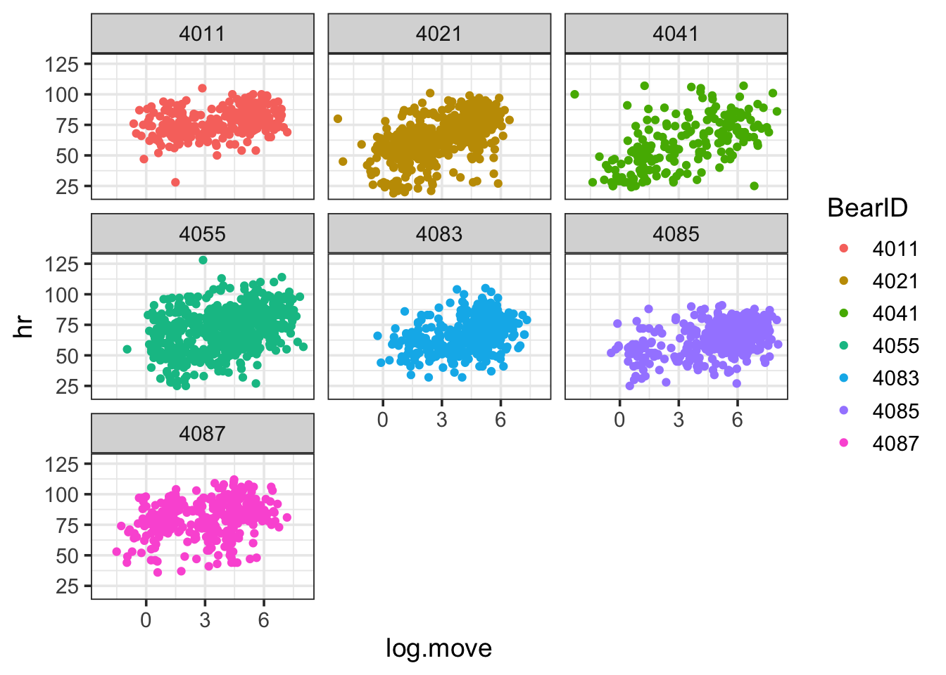
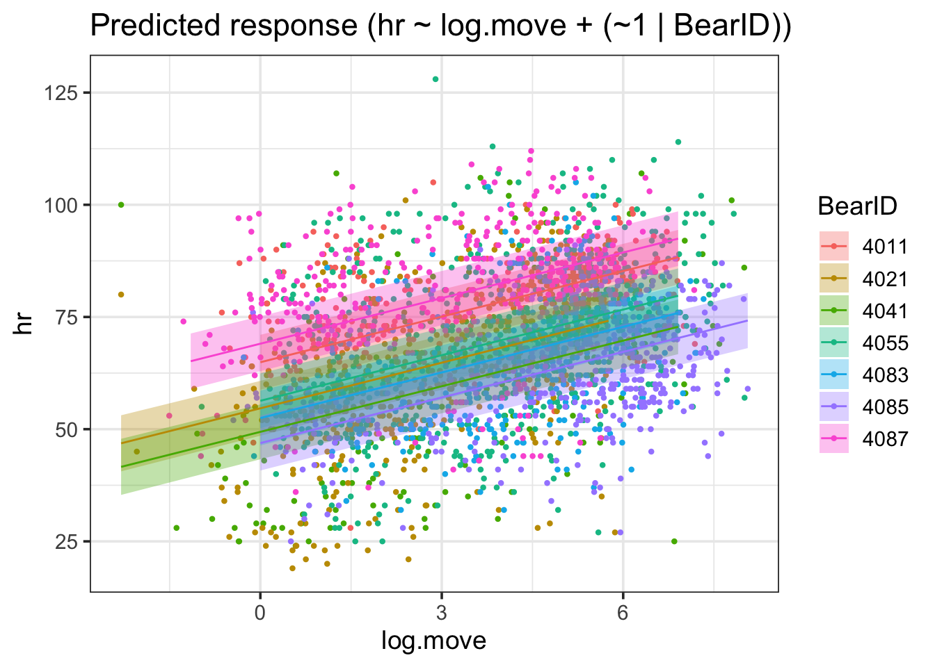
Lots going on here! To begin our exploration of variable intercept models, we’ll look at how heart rate is a function of log movement. We can visualize this, and also look at how different things are from bear-to-bear. We will use the variable BearIDYear and assume that measurements within a bear are independent of one another after we account for this variance component.
bear_base <-ggplot(bearmove,aes(y = hr, x = log.move, color = BearID)) +geom_point() +facet_wrap(vars(BearID)) bear_base
OK, we can see that the data bounces around from bear to bear. Maybe the slope does to? Who’s to say! Yet… We can ponder an initial model that accounts for this non-independence where Bear is a random effect. We sample the same bears over time, and as such, there might be a bear effect on heart rate (I mean, not all bears are created equal).
THINK: Is it reasonable to assume endogeneity?
1.1 Fitting and Evaluating a Variable Intercept Model
We’ll work with lme4 to fit a variable intercept model. Note, glmmTMB will have the same syntax, and many of the same workflows.
library(lme4)
Loading required package: Matrix
bear_int <-lmer(hr ~ log.move + (1|BearID), data = bearmove)
Great! Let’s look at whether we can use this model.
library(performance)
Warning: package 'performance' was built under R version 4.2.3
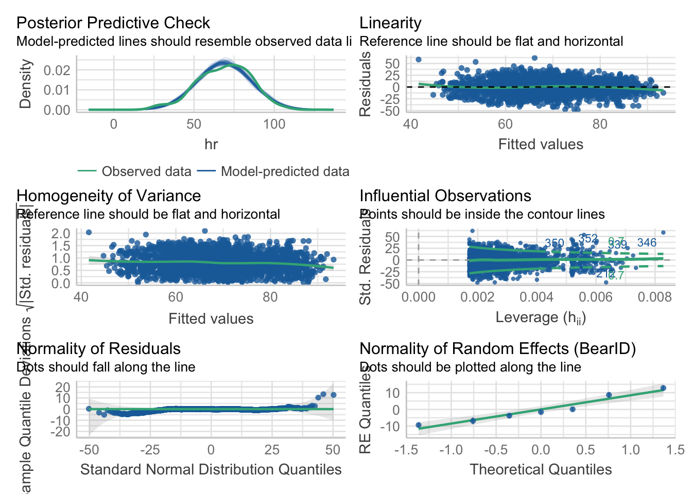
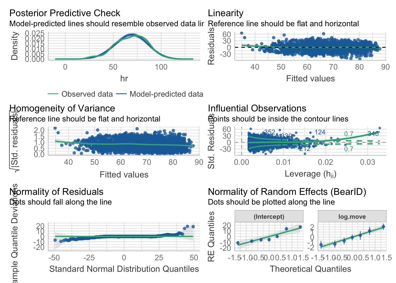
check_model(bear_int)
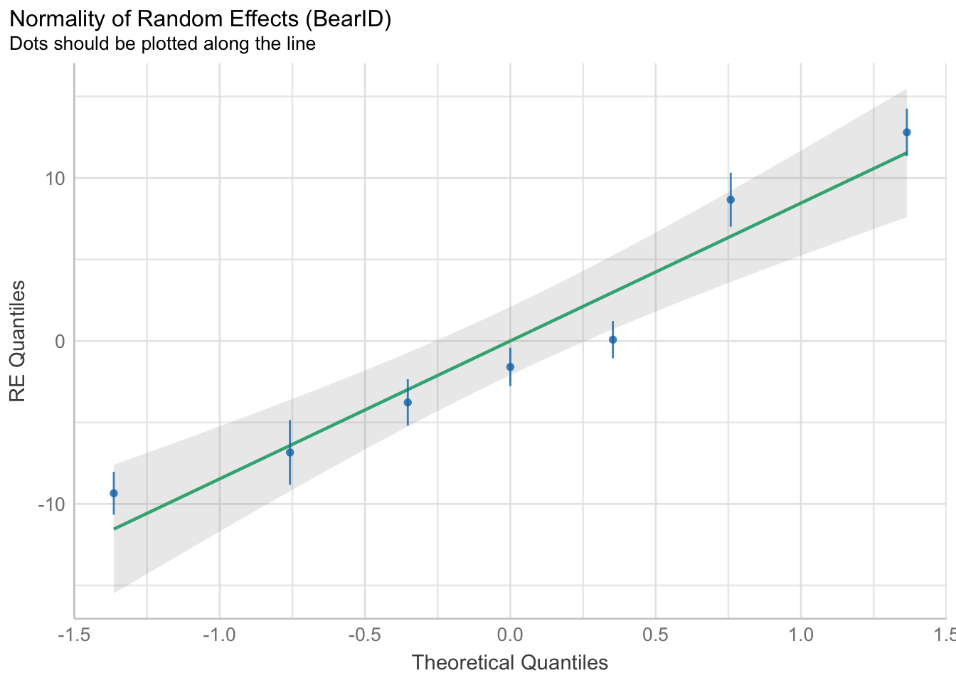
Looking at this overview, things look pretty good! The big new bit is checking the normality of the random effects here.
We can look at our outputs in a number of ways. Let’s look at the summary() output first.
summary(bear_int)
Linear mixed model fit by REML ['lmerMod']
Formula: hr ~ log.move + (1 | BearID)
   Data: bearmove

REML criterion at convergence: 22537

Scaled residuals:
    Min      1Q  Median      3Q     Max
-3.4210 -0.6341  0.0124  0.6749  4.3851

Random effects:
 Groups   Name        Variance Std.Dev.
 BearID   (Intercept)  65.56    8.097
 Residual             199.01   14.107
Number of obs: 2768, groups:  BearID, 7

Fixed effects:
            Estimate Std. Error t value
(Intercept)   56.243      3.118   18.04
log.move       3.388      0.139   24.37

Correlation of Fixed Effects:
         (Intr)
log.move -0.167
One - note it tells us we have convergence. This is key. Now, we can see information on the variance and SD of the random effects, and estimated of the fixed effects. We can also see this with broom.mixed::tidy(). The broom.mixed package is the mixed model extension of broom. It was forked off as there are some specific things with REs that don’t fit into the general output of broom.
library(broom.mixed)tidy(bear_int)
# A tibble: 4 × 6
  effect   group    term            estimate std.error statistic
  <chr>    <chr>    <chr>              <dbl>     <dbl>     <dbl>
1 fixed    <NA>     (Intercept)        56.2      3.12       18.0
2 fixed    <NA>     log.move            3.39     0.139      24.4
3 ran_pars BearID   sd__(Intercept)     8.10    NA          NA
4 ran_pars Residual sd__Observation    14.1     NA          NA
We see the same info, summarized a bit more neatly. If we wanted CI, we can use confint()
This is going to be easier to turn into a plot. There’s a great easystats library called modelbased that works much like performance. It has a few tools for visualization.
library(modelbased)
Warning: package 'modelbased' was built under R version 4.2.3
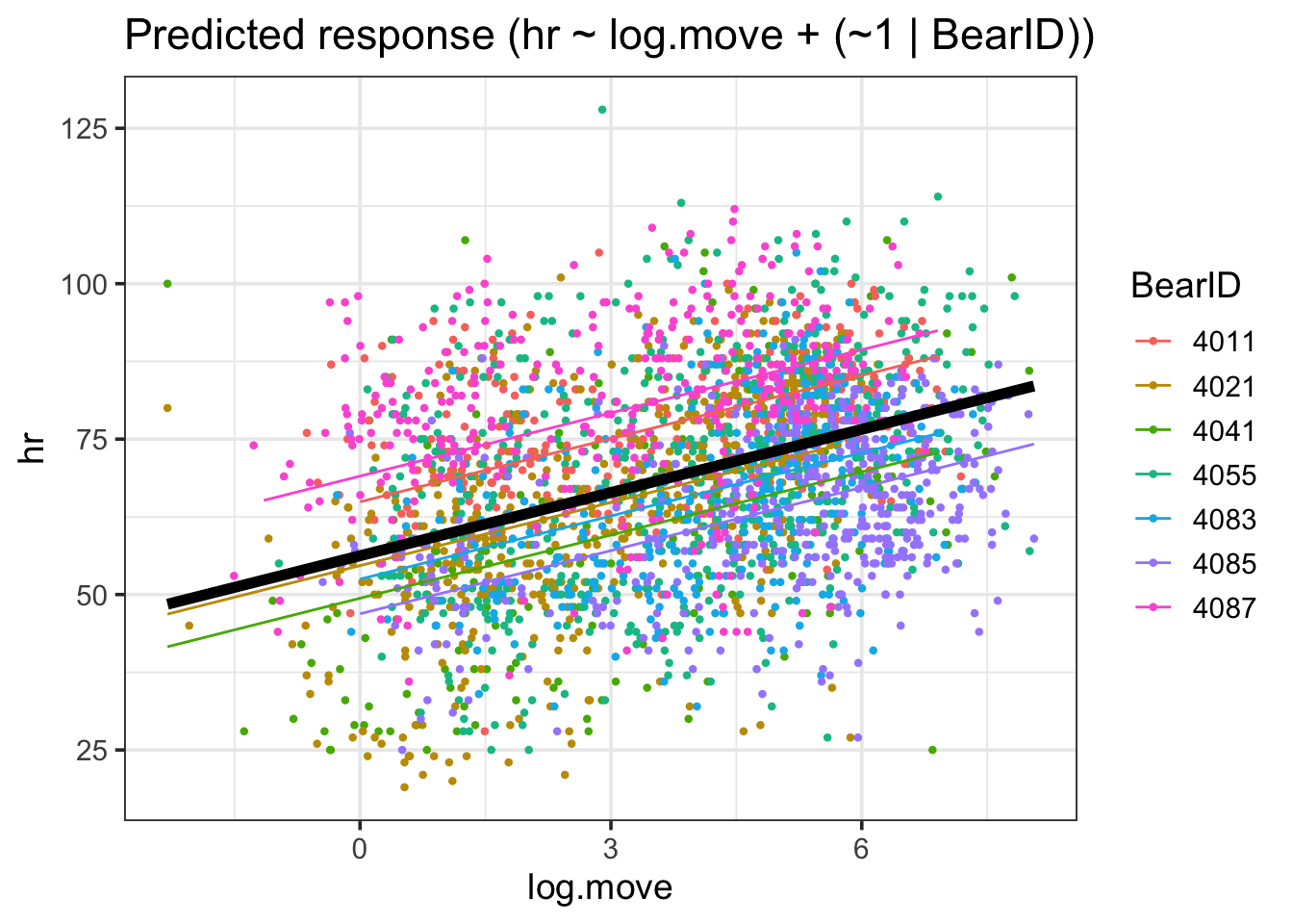
Now, one CAN use the outputs of different tidiers from above to build visualizations from scratch. It takes some work and reshaping. Perhaps it will be an “impress yourself” somewhere. For visualization, I’m a big fan of two things. First is estimate_relation() from modelbased and second it getting simulations from merTools::predictInterval(). We’ll stick with the former for the moment.
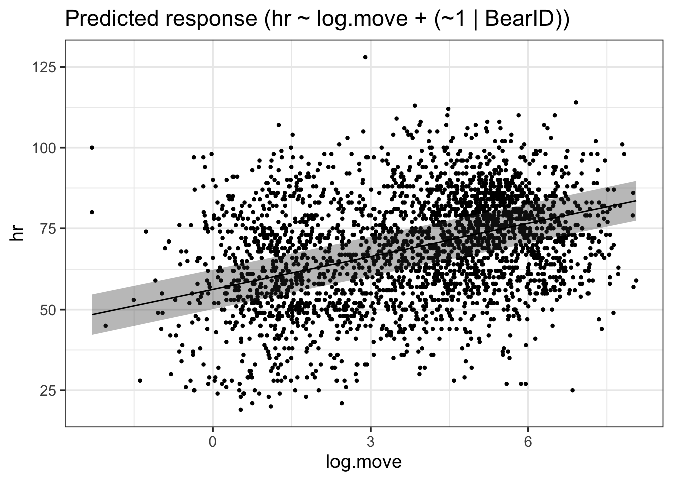
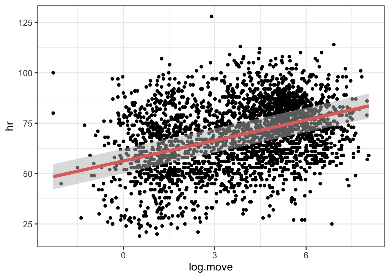
First up, do you want to look at just the marginal (fixed) effects?
estimate_relation(bear_int) |>plot()
There you go. All of the data with the FE through it. If you wanted to be more detailed, you can use the output to generate your own plot.
Consider the data set birdmalariaO in the Data4Ecologists library. These data are associated with the following paper: Asghar, M., Hasselquist, D., Hansson, B., Zehtindjiev, P., Westerdahl, H., & Bensch, S. (2015). Hidden costs of infection: chronic malaria accelerates telomere degradation and senescence in wild birds. Science, 347(6220), 436-438.
If we assess OffBTL - Offspring ealy-life telomere length (at 9 day age) - as a measure of fitness, how does mother’s age - mage - affect fitness, given that dam is mother id and brood is brood id (one mother can have many broods).
Now, consider not just mother’s age, but also mother’s malarial status - mmal. Note, you will have to make this a character.
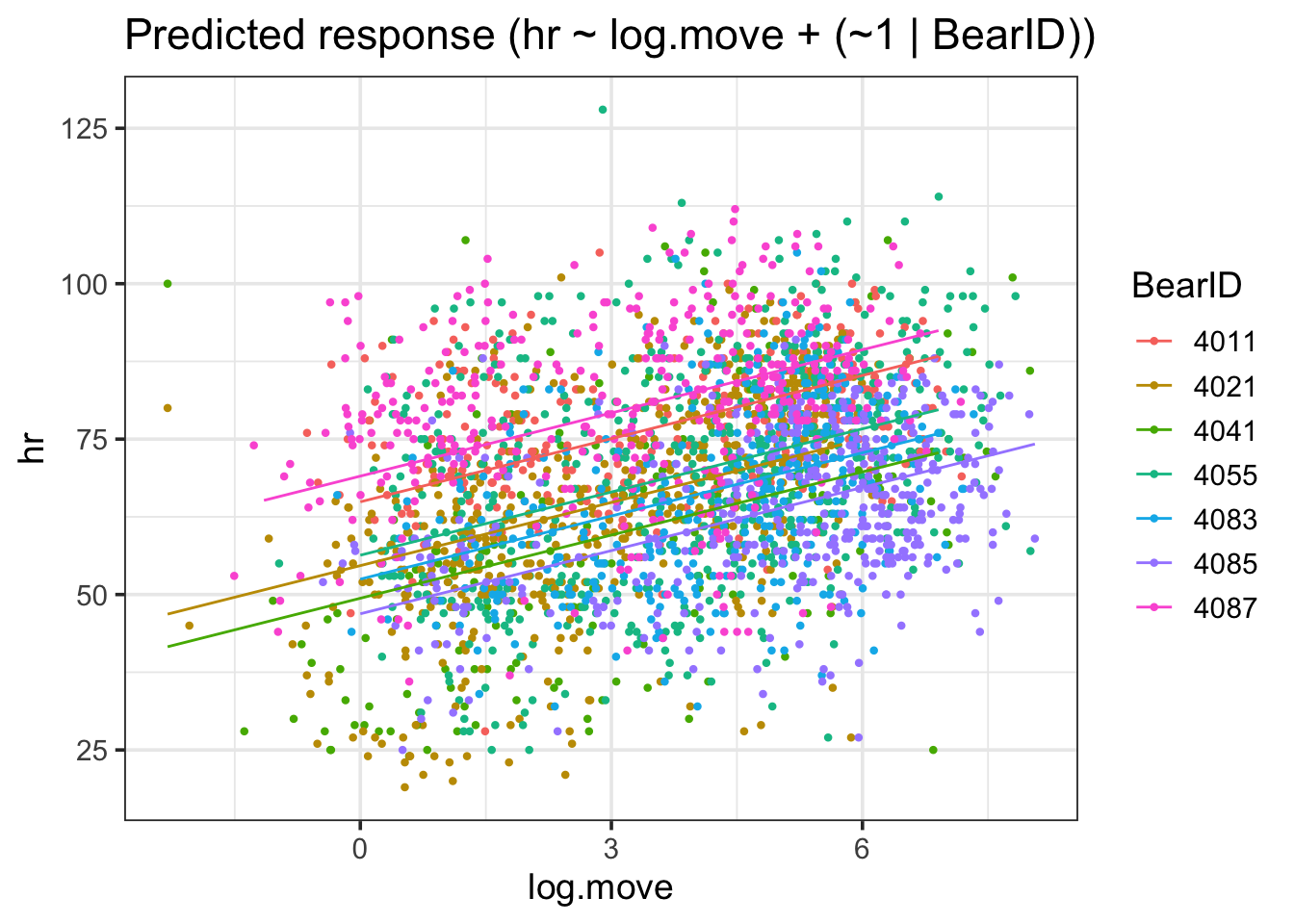
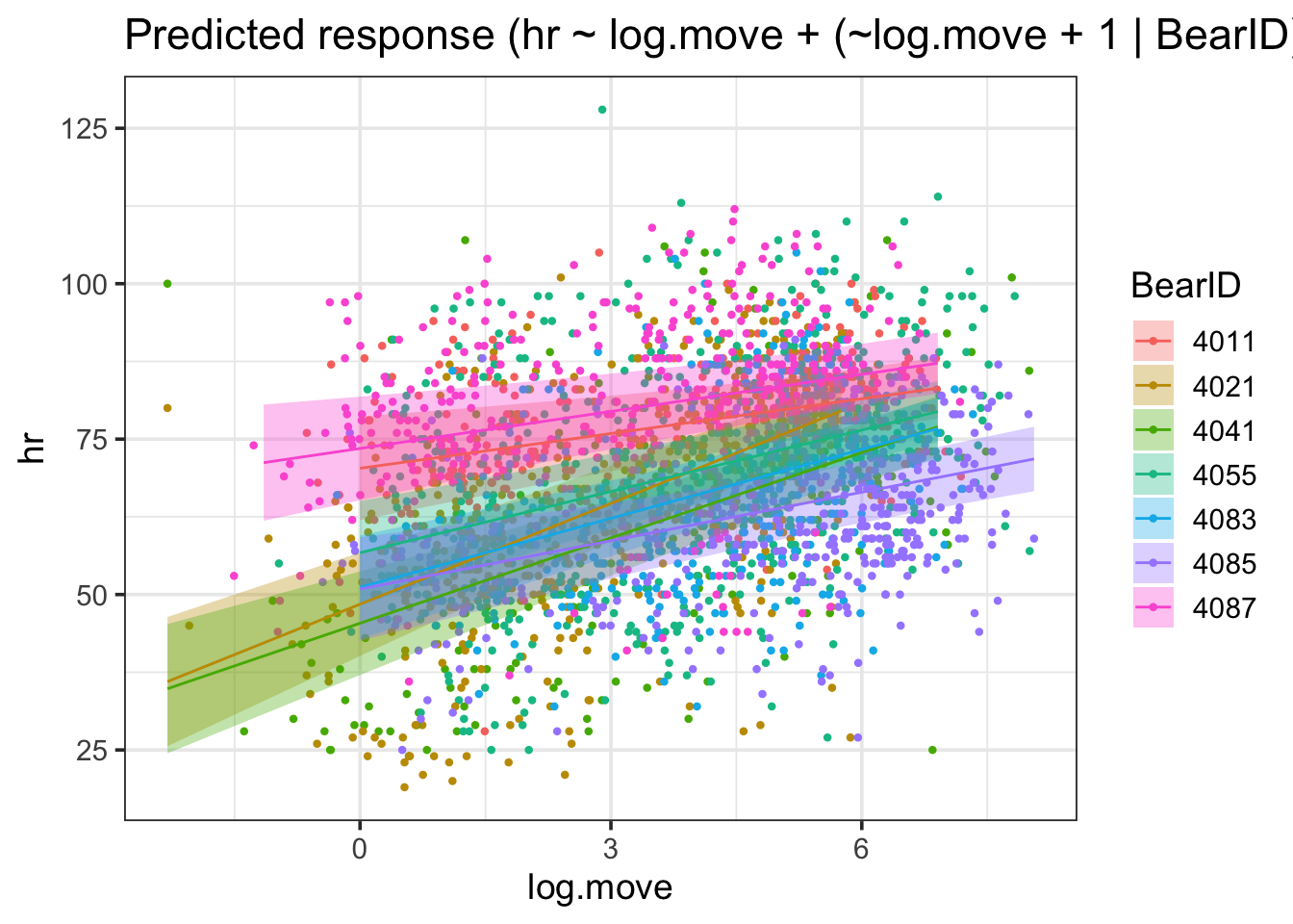
Back to bears, what if movement’s effect varied on heart rate by bear? Some are strong, some not so much… Might we have a variable slope?
bear_base
We can examine this with a variable-slope variable-intercept model.
bear_slope_int <-lmer(hr ~ log.move + (log.move +1|BearID), data = bearmove)
As before, we can examine assumptions
check_model(bear_slope_int)
There are some potential footballs in our HOV, and the QQ is a little funky, but largely this looks OK (for fun, try a DHARMa quantile residuals plot).
We can look at coefficients
tidy(bear_slope_int)
# A tibble: 6 × 6
  effect   group    term                      estimate std.error statistic
  <chr>    <chr>    <chr>                        <dbl>     <dbl>     <dbl>
1 fixed    <NA>     (Intercept)                 56.6       4.25      13.3
2 fixed    <NA>     log.move                     3.34      0.537      6.23
3 ran_pars BearID   sd__(Intercept)             11.1      NA         NA
4 ran_pars BearID   cor__(Intercept).log.move   -0.814    NA         NA
5 ran_pars BearID   sd__log.move                 1.37     NA         NA
6 ran_pars Residual sd__Observation             13.9      NA         NA
And, indeed, all terms suggest they should be included in the model. Note the correlation between random slopes and intercepts, FYI.
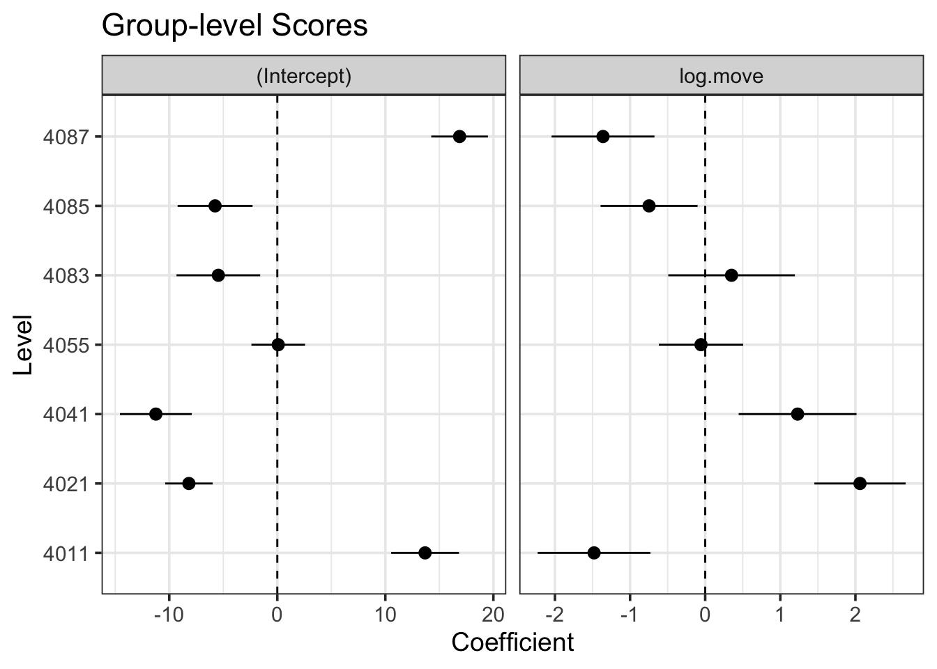
We can look at our REs
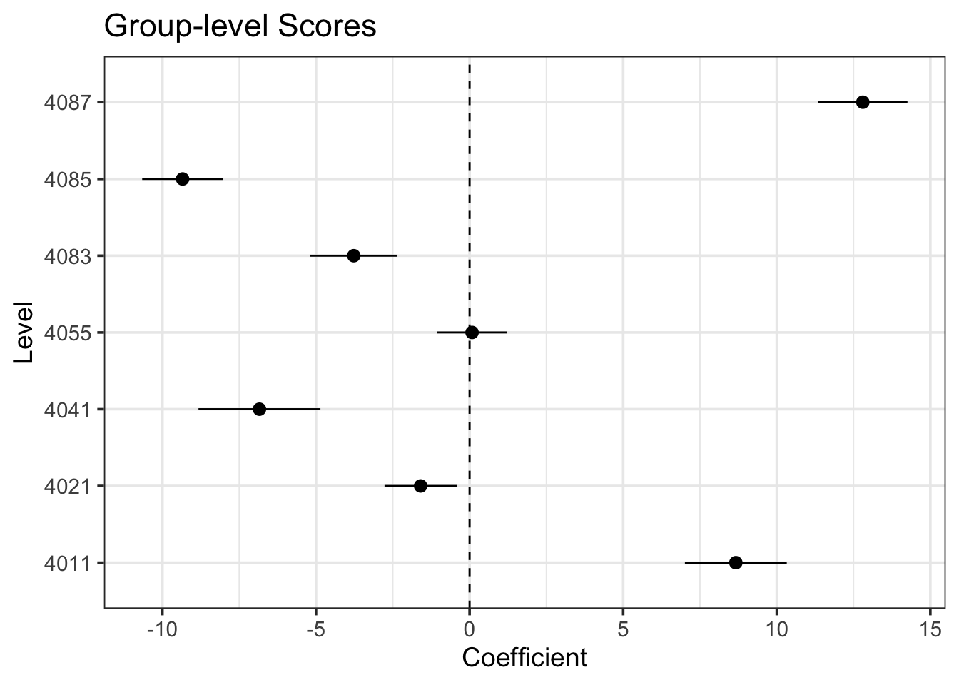
estimate_grouplevel(bear_slope_int) |>plot()
I find this one fairly interesting, as we can see both that there were some that were further away from the mean slope than others - but not too far when compared to the magnitude of the slope. No outright sign flips, etc.
We can visually see here that while slopes do vary, it’s not by a heck of a lot. But, this variability can be important, particularly with respect to proper CIs.
2.1 Example
Let’s just back into birdmalariaO If we assess OffBTL - Offspring ealy-life telomere length (at 9 day age) - as a measure of fitness, how does mother’s age - mage - and malarial status mmal - affect fitness, given that dam is mother id and brood is brood id (one mother can have many broods).
Should there be a mage*mmal interaction? What do you think, after thinking about the biology and looking at the data?
Now, where should the RE go? Begin with one where the effects of malaria vary by brood. After all, different years might experience different strains or severity.
Note, for multiple predictors, use estimate_relation() instead of estimate_prediction(). You might also want to take it, turn it into a tibble, and plot instead of relying on plot()
Once you are comfortable with results, fit a model where mage’s effect varies by dam as well. Birds might vary in how age-related maternal effects influence fitness.
But - what happens? This is where we grapple with some of the complexity. Let’s talk about RE structure and look at those warning messages carefully.
3. Hierarchical Models
Back to bears, our fuzzy bears have some properties that do not vary from individual to individual. And some of which could be linked right to heart rate. For example, does Sex change bear heart rate?
I’ll leave it as an exercise for you to evalute assumptions and see if the R2. But, what’s great is that we can use emmeans to actually ask if the sexes are different, just as before.
library(emmeans)emmeans(bear_hier, ~ Sex)
 Sex emmean   SE   df lower.CL upper.CL
 F     72.9 3.10 5.83     65.3     80.6
 M     64.4 3.58 5.91     55.6     73.2

Degrees-of-freedom method: kenward-roger
Confidence level used: 0.95
Note that it mentions DF used for calculating those CIs. These are different methods for calculating those DF, and the K-W method is fairly standard. We can then do a contrast as usual.
 contrast estimate   SE   df lower.CL upper.CL
 F - M        8.57 4.71 4.97    -3.55     20.7

Degrees-of-freedom method: kenward-roger
Confidence level used: 0.95
So, while our estimate is that females have a higher heart rate, there is considerable variability, or low precision, in our estimate. We cannot reject the idea that sex does not matter here.
4. GLMMs
Some times, our response variables are not normal. For example, in the RIKZ beach data, richness is likely to be Poisson distributed. Or negative binomial. Either way, it’s count. Let’s look at that with a variable random-slope model where NAP determines richness, but it’s effect varies by beach. To do this with a poisson, we’ll need glmer() the generalized implementation of lmer()
# Start with the data, and make a character for BeachRIKZdat <- RIKZdat |>mutate(Beach =as.character(Beach))rikz_mod <-glmer(Richness ~ NAP + (NAP +1| Beach),family =poisson(link ="log"),data = RIKZdat)
This works beautifully. Now, while we should look at our predictions, our RE QQ plots, and our outliers - we also have to look at quantile residuals. We can also check overdispersion.
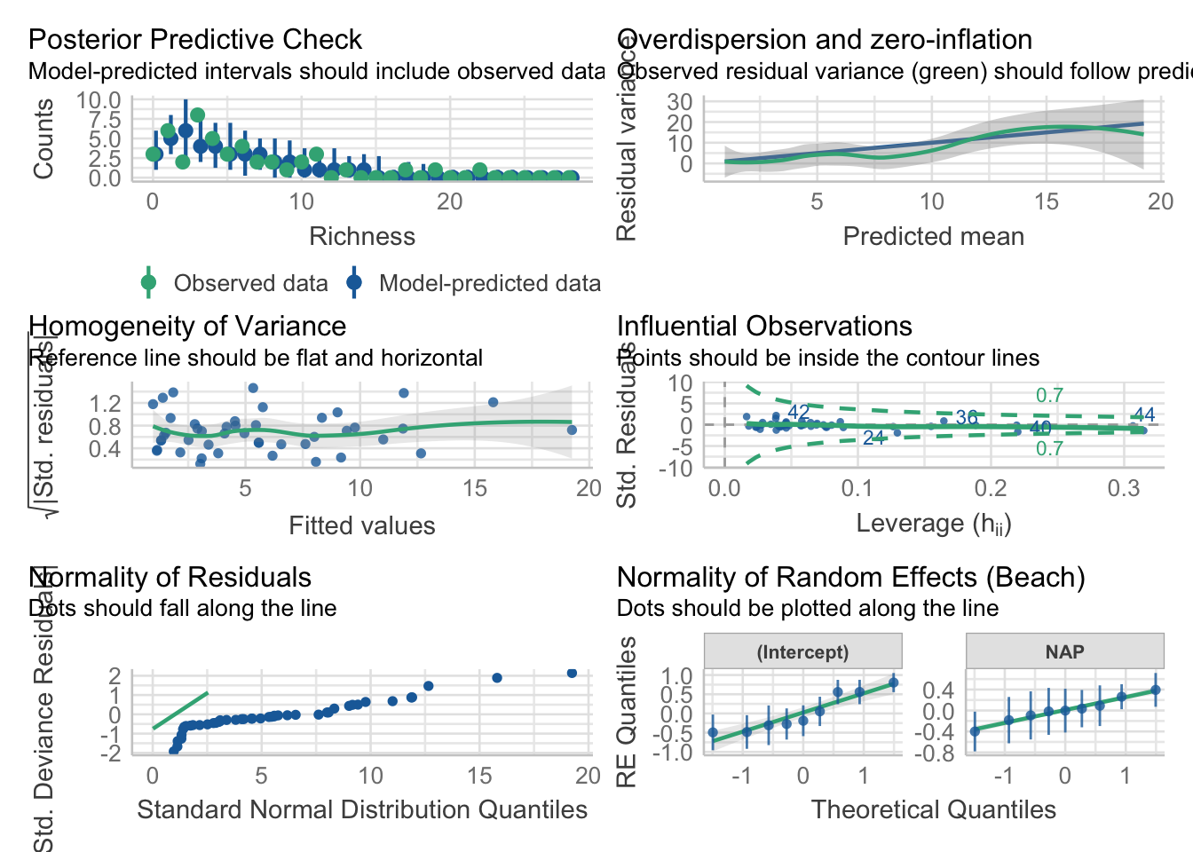
check_model(rikz_mod)
Most things look pretty good here. Our overdispersion is a bit wonky, but we can check that in more detail with quantile residuals.
library(DHARMa)
This is DHARMa 0.4.6. For overview type '?DHARMa'. For recent changes, type news(package = 'DHARMa')
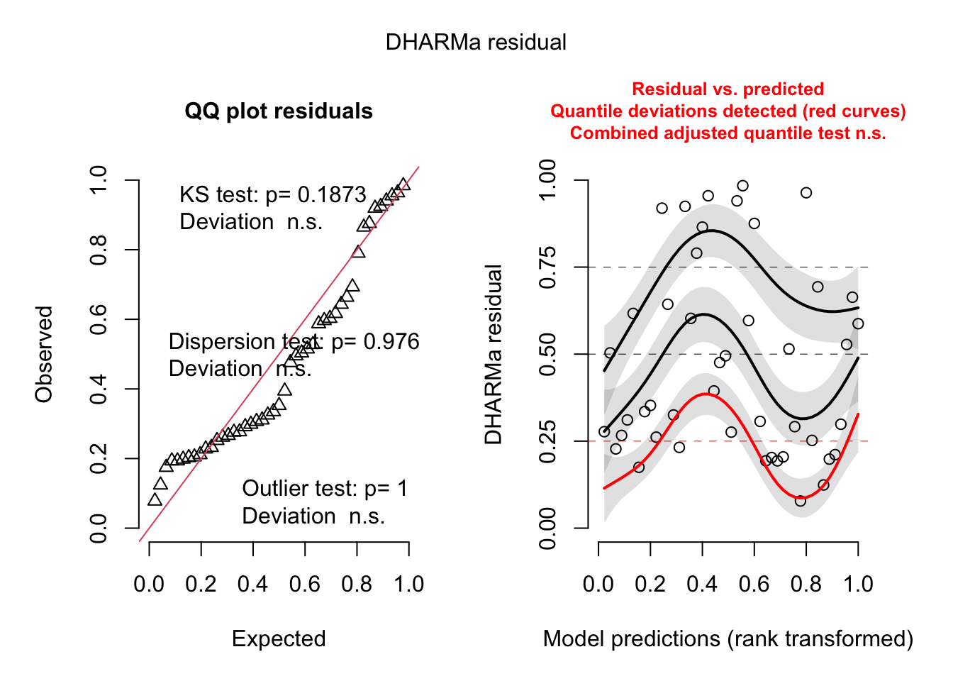
simulateResiduals(rikz_mod) |>plot()
This again…. actually is fine. We still see that wiggliness, though, in the rank prediction against residual. If one was really worried about that, we could use a negative binomial error. Here, though, be dragons, and we’ll need to switch to glmmTMB.
library(glmmTMB)
Warning in checkDepPackageVersion(dep_pkg = "TMB"): Package version inconsistency detected.
glmmTMB was built with TMB version 1.9.4
Current TMB version is 1.9.6
Please re-install glmmTMB from source or restore original 'TMB' package (see '?reinstalling' for more information)
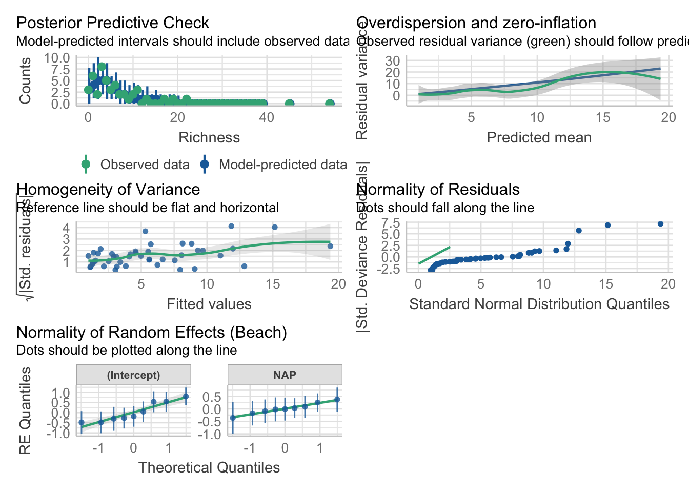
`check_outliers()` does not yet support models of class `glmmTMB`.
Same.
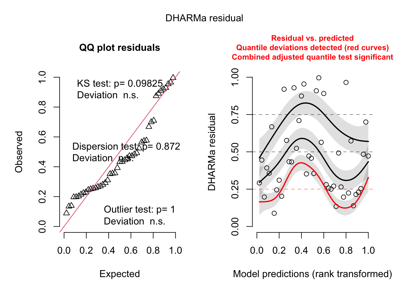
simulateResiduals(rikz_nb) |>plot()
qu = 0.25, log(sigma) = -3.495193 : outer Newton did not converge fully.
qu = 0.25, log(sigma) = -3.510995 : outer Newton did not converge fully.
Same. One may well ask, did we need the nbinom2 here?
summary(rikz_nb)
 Family: nbinom2  ( log )
Formula:          Richness ~ NAP + (NAP + 1 | Beach)
Data: RIKZdat

     AIC      BIC   logLik deviance df.resid
   220.7    231.5   -104.3    208.7       39

Random effects:

Conditional model:
 Groups Name        Variance Std.Dev. Corr
 Beach  (Intercept) 0.25773  0.5077
        NAP         0.08211  0.2865   0.20
Number of obs: 45, groups:  Beach, 9

Dispersion parameter for nbinom2 family ():  103

Conditional model:
            Estimate Std. Error z value Pr(>|z|)
(Intercept)   1.6935     0.1864   9.086  < 2e-16 ***
NAP          -0.6076     0.1370  -4.436 9.16e-06 ***
---
Signif. codes:  0 '***' 0.001 '**' 0.01 '*' 0.05 '.' 0.1 ' ' 1
With a fairly substantial dispersion, perhaps. We can also visualize to see how this might change our inference, or look at comparisons of coefficients.
tidy(rikz_mod)
# A tibble: 5 × 7
  effect   group term                 estimate std.error statistic   p.value
  <chr>    <chr> <chr>                   <dbl>     <dbl>     <dbl>     <dbl>
1 fixed    <NA>  (Intercept)             1.69      0.187      9.07  1.18e-19
2 fixed    <NA>  NAP                    -0.607     0.137     -4.42  9.81e- 6
3 ran_pars Beach sd__(Intercept)         0.513    NA         NA    NA
4 ran_pars Beach cor__(Intercept).NAP    0.180    NA         NA    NA
5 ran_pars Beach sd__NAP                 0.299    NA         NA    NA
tidy(rikz_nb)
# A tibble: 5 × 8
  effect   component group term           estimate std.error statistic   p.value
  <chr>    <chr>     <chr> <chr>             <dbl>     <dbl>     <dbl>     <dbl>
1 fixed    cond      <NA>  (Intercept)       1.69      0.186      9.09  1.03e-19
2 fixed    cond      <NA>  NAP              -0.608     0.137     -4.44  9.16e- 6
3 ran_pars cond      Beach sd__(Intercep…    0.508    NA         NA    NA
4 ran_pars cond      Beach sd__NAP           0.287    NA         NA    NA
5 ran_pars cond      Beach cor__(Interce…    0.202    NA         NA    NA
We can see why plots looked so similar - we get the same coefficients more or less. So, while the NB is more flexible, it might not be as big if an issue here.
This is actually a great place to introduce merTools::predictInterval() which allows one to generate intervals around fit due to fit error, random effects, or RE + residual error (i.e., fill prediction intervals).
library(merTools)
Loading required package: arm
Loading required package: MASS
Attaching package: 'MASS'
The following object is masked from 'package:dplyr':

    select
arm (Version 1.13-1, built: 2022-8-25)
Working directory is /Users/jebyrnes/Dropbox (Byrnes Lab)/Classes/biol_607_biostats/lab
Attaching package: 'arm'
The following object is masked from 'package:modelbased':

    standardize
The following object is masked from 'package:performance':

    display
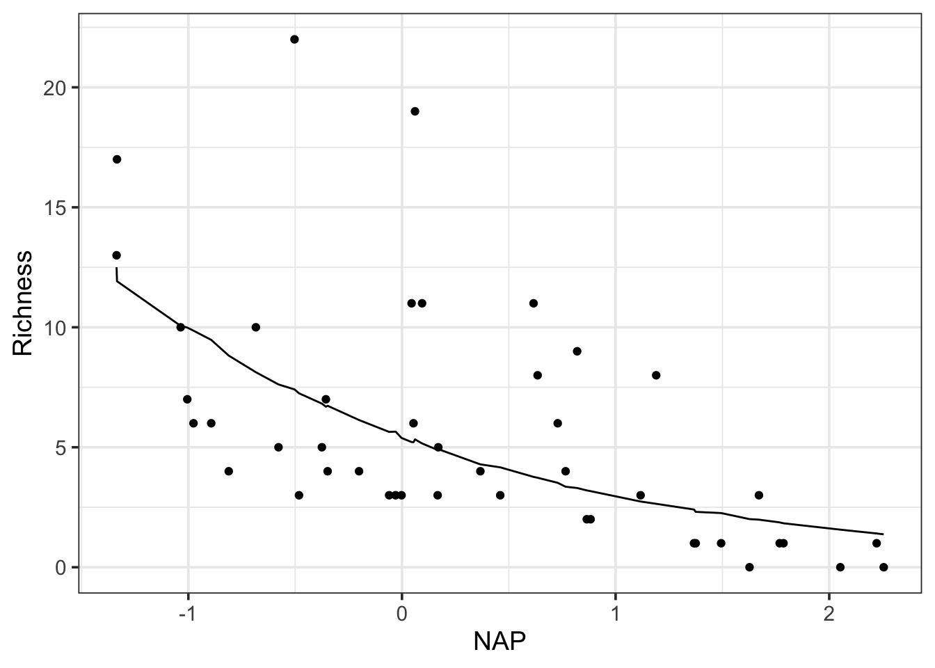
pred <-predictInterval(rikz_mod, which ="fixed",n.sims =10000) |>cbind(RIKZdat)
Warning in predictInterval(rikz_mod, which = "fixed", n.sims = 10000):
Prediction for NLMMs or GLMMs that are not mixed binomial regressions is not
tested. Sigma set at 1.
Warning: executing %dopar% sequentially: no parallel backend registered
ggplot(pred,aes(x = NAP, y = Richness)) +geom_point() +geom_line(aes(y =exp(fit)))
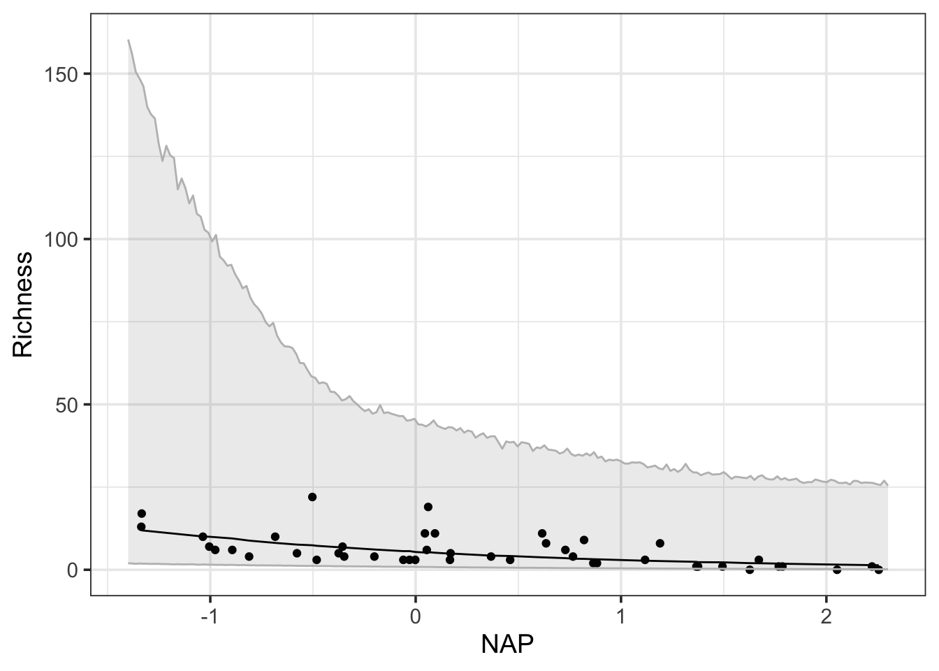
Note, this line is janky because it’s from simulations, and those aren’t 100% simple with a complex model structure. You could just start all of this using estimate_relation() or somesuch for a smoother fit. But where predictInterval shines is the creation of prediction intervals using full RE and residual structure. However, we need to select the extreme upper and lower values, otherwise we’ll just plot the values for each beach.