library(readr)
library(dplyr)

library(performance)
library(car)
library(broom)
library(modelr)
library(emmeans)

library(ggplot2)
library(GGally)
library(visreg)
library(piecewiseSEM)

theme_set(theme_bw(base_size = 14))Complex Linear Models
For today, let’s start with some standard libraries for these analyses.
1. Many Categorical Varibles
We’ll work with the zooplankton depredation dataset for two-way linear model with categorical predictors. This is a blocked experiment, so, each treatment is in each block just once.
zooplankton <- read_csv("./data/18e2ZooplanktonDepredation.csv") Rows: 15 Columns: 3
── Column specification ────────────────────────────────────────────────────────
Delimiter: ","
chr (1): treatment
dbl (2): zooplankton, block
ℹ Use `spec()` to retrieve the full column specification for this data.
ℹ Specify the column types or set `show_col_types = FALSE` to quiet this message.ggplot(data = zooplankton,
aes(x = treatment, y = zooplankton)) +
geom_boxplot()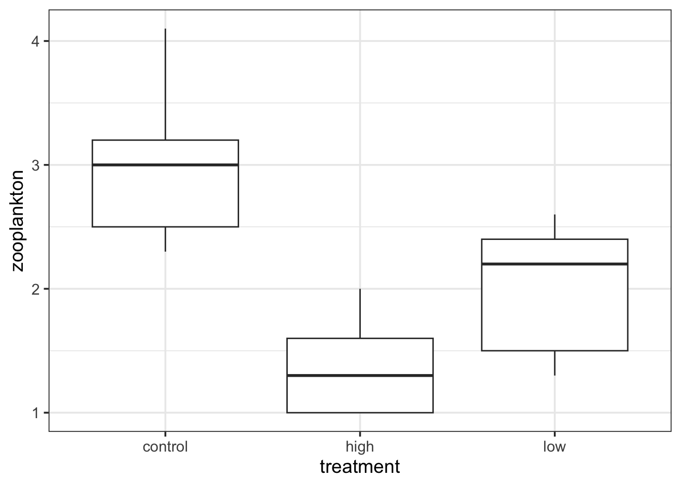
ggplot(data = zooplankton,
       aes(x = block, y = zooplankton)) +
  geom_boxplot()
Warning: Continuous x aesthetic
ℹ did you forget `aes(group = ...)`?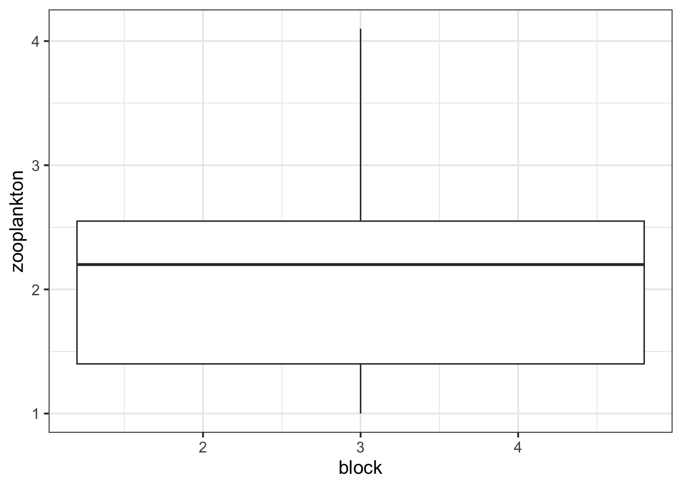
Oh. That’s odd. What is up with block? AH HA! It’s continuous. We need to make it discrete to work with it.
zooplankton <- zooplankton |>
  mutate(block = as.character(block))

ggplot(data = zooplankton,
       aes(x = block, y = zooplankton)) +
  geom_boxplot()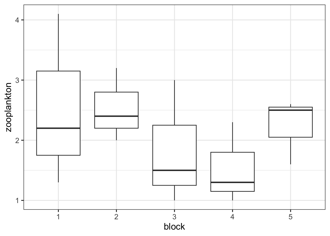
There we go. Always check!
1.1 Fit and Assumption Evaluation
Fit is quite easy. We just add one more factor to an lm model!
zooplankton_lm <- lm(zooplankton ~ treatment + block,
                     data = zooplankton)
We then evaluate residuals almost as usual…
library(performance)
check_model(zooplankton_lm)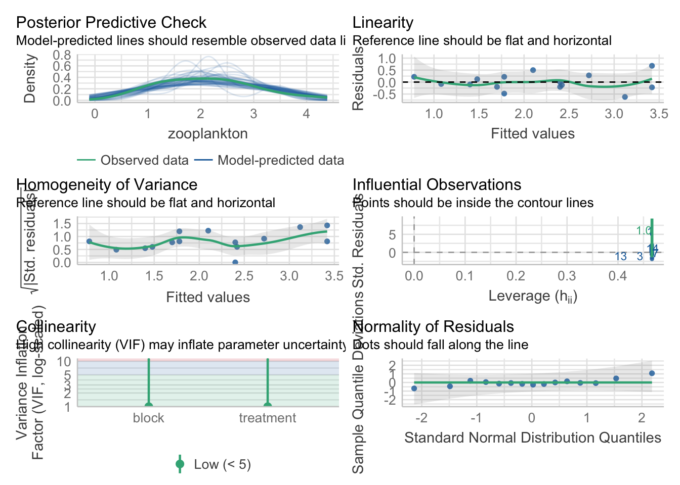
We want to look more deeply by fitted versus residuals to inspect for nonadditivity. Let’s check it out.
check_model(zooplankton_lm, check = "linearity") |> plot()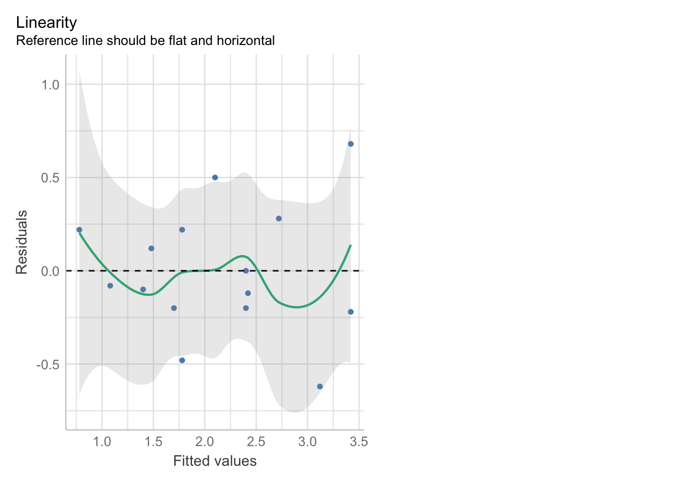
Looks good!
1.2 Coefficients
Let’s look at the coefs!
tidy(zooplankton_lm)# A tibble: 7 × 5
term estimate std.error statistic p.value
<chr> <dbl> <dbl> <dbl> <dbl>
1 (Intercept) 3.42e+ 0 0.313 1.09e+ 1 0.00000433
2 treatmenthigh -1.64e+ 0 0.289 -5.67e+ 0 0.000473
3 treatmentlow -1.02e+ 0 0.289 -3.52e+ 0 0.00781
4 block2 9.57e-16 0.374 2.56e-15 1.00
5 block3 -7.00e- 1 0.374 -1.87e+ 0 0.0979
6 block4 -1.00e+ 0 0.374 -2.68e+ 0 0.0281
7 block5 -3.00e- 1 0.374 -8.03e- 1 0.445 This is still a little odd, though, as our treatments are evaluated in block 1 control. To truly get just the treatment effect, we need to look at the estimated marginal means - the emmeans! The big thing about emmeans is that it creates a reference grid based on the blocks. It then calculates the treatment effect averaged over all blocks, rather than just in block 1.
library(emmeans)

zoop_em <- emmeans(zooplankton_lm, ~treatment)

zoop_em
treatment emmean SE df lower.CL upper.CL
control 3.02 0.205 8 2.548 3.49
high 1.38 0.205 8 0.908 1.85
low 2.00 0.205 8 1.528 2.47
Results are averaged over the levels of: block
Confidence level used: 0.95 1.3 Evaluating treatment differences
Here, emmeans gets interesting.
contrast(zoop_em, method = "pairwise") |>
  confint()
contrast estimate SE df lower.CL upper.CL
control - high 1.64 0.289 8 0.813 2.467
control - low 1.02 0.289 8 0.193 1.847
high - low -0.62 0.289 8 -1.447 0.207
Results are averaged over the levels of: block
Confidence level used: 0.95
Conf-level adjustment: tukey method for comparing a family of 3 estimates Note the message that we’ve averaged over the levels of block. You can do any sort of posthoc evaluation (query your model!) as you wanted before. And, you could have done the same workflow for block as well.
1.4 Faded Examples
Given then similarity with models from last week, let’s just jump right into two examples, noting a key difference or two here and there.
To start with, let’s look at gene expression by different types of bees.
bees <- read.csv("./data/18q07BeeGeneExpression.csv")

#Visualize
________(data=____,
         aes(x = type, y = Expression)) +
  _________()

#fit
bee_lm <- __(______ ~ ______ + _____, data=________)

#assumptions
________(______)

#pairwise comparison
emmeans(__________, spec = ~ ________) |>
  contrast(method = "pairwise") |>
  confint()
Wow, not that different, save adding one more term and the residualPlots.
OK, one more…. repeating an experiment in the intertidal?
intertidal <- read.csv("./data/18e3IntertidalAlgae.csv")

#Visualize
ggplot(data = _____________,
       _____ = ______(x = herbivores, y = sqrtarea)) +
  _____________()

#fit
intertidal_lm <- __(______ ~ ______ + _____, data=________)

#assumptions
________(______)

#pairwise comparison
emmeans(__________, spec = ~ ________) |>
  contrast(method = "___________") |>
  ________()
Did that last one pass the test of non-additivity?
2. Mixing Categorical and Continuous Variables
Combining categorical and continuous variables is not that different from what we have done above. To start with, let’s look at the neanderthal data from class.
neand <- read.csv("./data/18q09NeanderthalBrainSize.csv")
head(neand)
lnmass lnbrain species
1 4.00 7.19 recent
2 3.96 7.23 recent
3 3.95 7.26 recent
4 4.04 7.23 recent
5 4.11 7.22 recent
6 4.10 7.24 recentWe can clearly see both the categorical variable we’re interested in, and the covariate.
To get a preliminary sense of what’s going on here, do some exploratory visualization with ggplot2 why doncha!
ggplot(data = neand,
       mapping = aes(x = lnmass, y = lnbrain,
                     color = species)) +
  geom_point() +
  stat_smooth(method = "lm")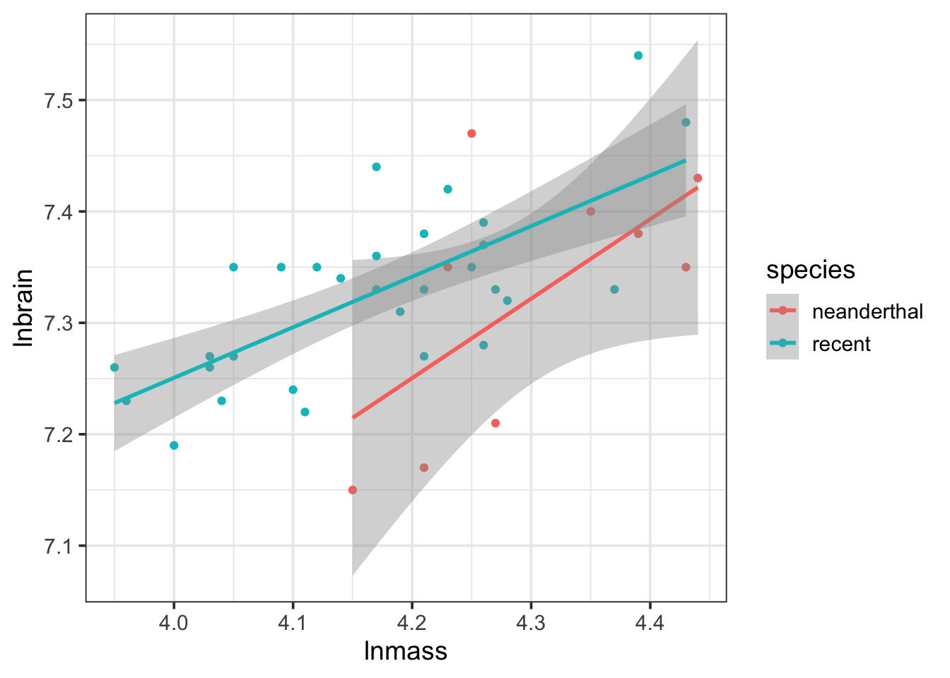
Now, the CIs are going to be off as this wasn’t all tested in the same model, but you begin to get a sense of whether things are parallel or not, and whether this covariate is important.
What other plots might you produce?
As this is a general linear model, good olde lm() is still there for us.
neand_lm <- lm(lnbrain ~ species + lnmass, data=neand)2.1 Testing Assumptions
In addition to the ususal tests, we need to make sure that the slopes really are parallel. We do that by fitting a model with an interaction and testing it (which, well, if there was and interaction, might that be interesting).
First, the usual
check_model(neand_lm)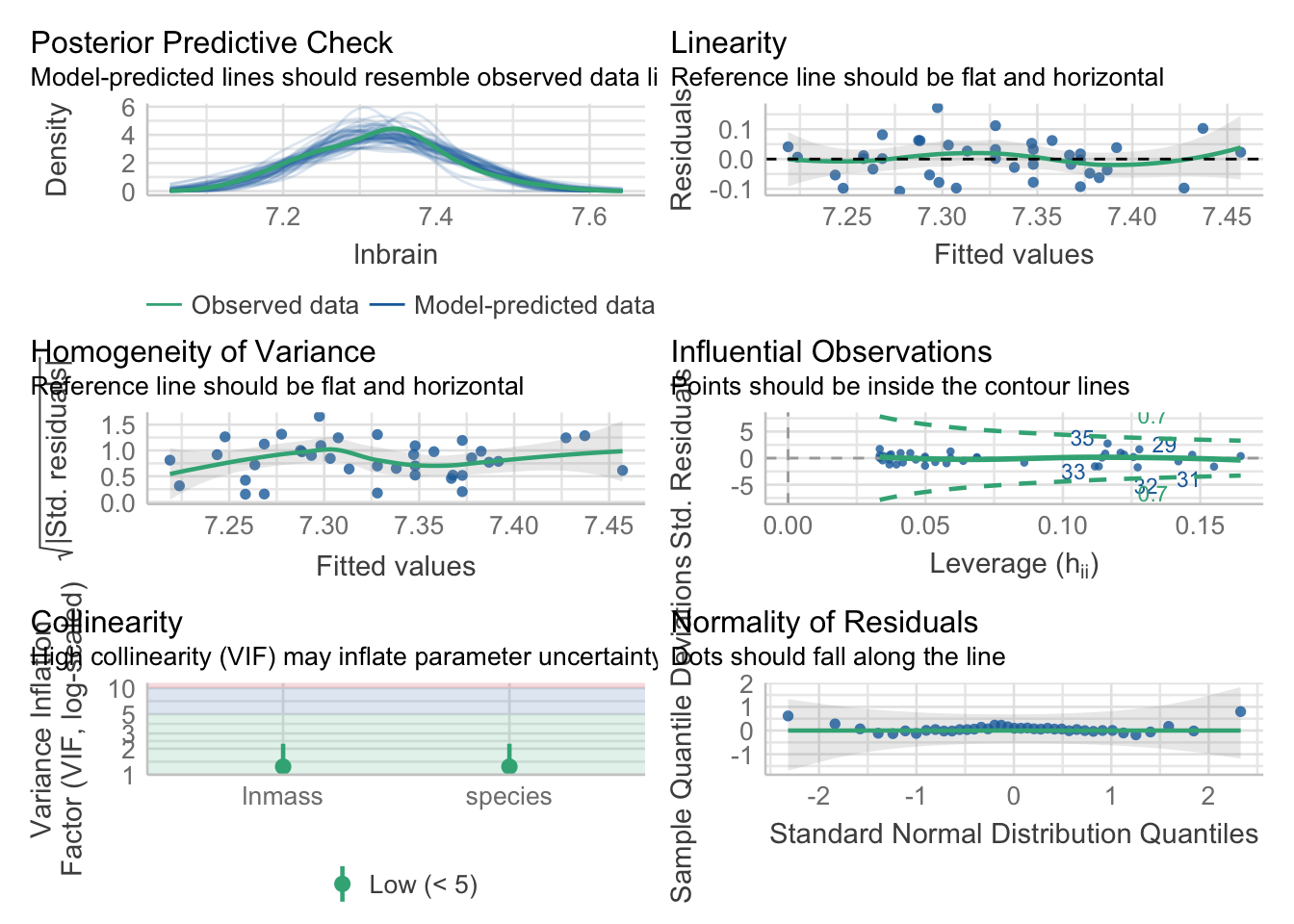
#And now look at residuals by group/predictors
library(car)
residualPlots(neand_lm, tests=FALSE)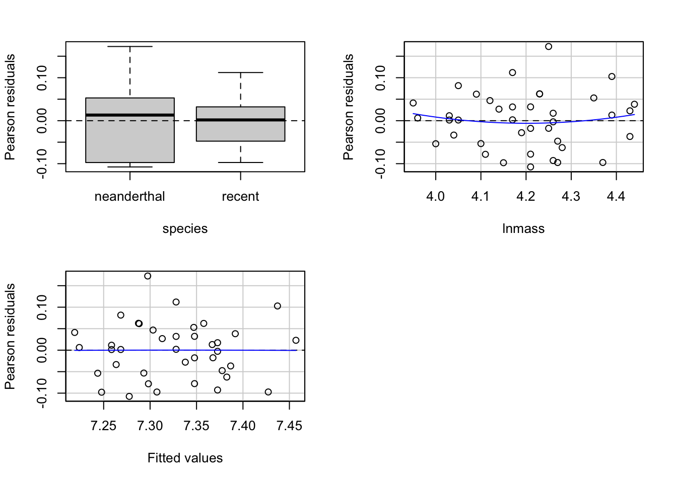
To test the parallel presumption
neand_int <- lm(lnbrain ~ species*lnmass, data=neand)

tidy(neand_int)
# A tibble: 4 × 5
term estimate std.error statistic p.value
<chr> <dbl> <dbl> <dbl> <dbl>
1 (Intercept) 4.25 0.977 4.35 0.000111
2 speciesrecent 1.18 1.06 1.11 0.274
3 lnmass 0.714 0.227 3.14 0.00340
4 speciesrecent:lnmass -0.259 0.248 -1.05 0.303 We can see that there is no interaction, and hence we are a-ok to proceed with the parallel lines model.
2.2 Assessing results
Now, let’s look at our coefficients
tidy(neand_lm)# A tibble: 3 × 5
term estimate std.error statistic p.value
<chr> <dbl> <dbl> <dbl> <dbl>
1 (Intercept) 5.19 0.395 13.1 2.74e-15
2 speciesrecent 0.0703 0.0282 2.49 1.75e- 2
3 lnmass 0.496 0.0917 5.41 4.26e- 6Everything looks like it matters. If you had wanted to do this with a centered covariate, how would things differ? Try it out.
Second, does our model explain much?
r2(neand_lm)# R2 for Linear Regression
R2: 0.449
adj. R2: 0.418Not bad - and both types agree fairly well.
Next, we might want to compare covariate adjusted groups and/or look at covariate adjusted means.
library(emmeans)
adj_means <- emmeans(neand_lm, specs = ~species)

#adjusted means
adj_means
species emmean SE df lower.CL upper.CL
neanderthal 7.272 0.02419 36 7.223 7.321
recent 7.342 0.01250 36 7.317 7.367
Confidence level used: 0.95 Nice! But, what if we wanted to know what value of the covariate we were using? To get those, we need to use say that we are using lnmass as a reference grid - i.e. we’re marginalizing over it.
avg_sp_means <- emmeans(neand_lm, ~species|lnmass)
avg_sp_meanslnmass = 4.198:
 species     emmean      SE df lower.CL upper.CL
 neanderthal  7.272 0.02419 36    7.223    7.321
 recent       7.342 0.01250 36    7.317    7.367

Confidence level used: 0.95 We can then use this for pairwise comparisons, etc.
#comparisons
contrast(avg_sp_means, method="pairwise") |>
  confint()
lnmass = 4.2:
contrast estimate SE df lower.CL upper.CL
neanderthal - recent -0.0703 0.0282 36 -0.128 -0.0131
Confidence level used: 0.95 You can also specify other levels of mass, if you are more interested in those for biological relevance. You can even specify multiple levels, or even a smooth curve and plot the results!
We can also see the estimates of the slopes for each species (which is more useful when there is an interaction - as summary is just fine without.)
#no interaction
emtrends(neand_lm, ~species, var = "lnmass")
species lnmass.trend SE df lower.CL upper.CL
neanderthal 0.496 0.0917 36 0.31 0.682
recent 0.496 0.0917 36 0.31 0.682
Confidence level used: 0.95 2.3 Visualization
Visualization is funny, as you want to make parallel lines and also get the CIs right. Rather than rely on ggplot2 to do this natively, we need to futz around a bit with generating predictions
neand_predict <- augment(neand_lm, interval="confidence")

head(neand_predict)
# A tibble: 6 × 11
lnbrain species lnmass .fitted .lower .upper .resid .hat .sigma .cooksd
<dbl> <chr> <dbl> <dbl> <dbl> <dbl> <dbl> <dbl> <dbl> <dbl>
1 7.19 recent 4 7.24 7.20 7.28 -0.0536 0.0860 0.0669 0.0222
2 7.23 recent 3.96 7.22 7.18 7.27 0.00624 0.114 0.0676 0.000425
3 7.26 recent 3.95 7.22 7.17 7.27 0.0412 0.122 0.0672 0.0202
4 7.23 recent 4.04 7.26 7.23 7.30 -0.0335 0.0637 0.0673 0.00611
5 7.22 recent 4.11 7.30 7.27 7.33 -0.0782 0.0394 0.0662 0.0196
6 7.24 recent 4.1 7.29 7.27 7.32 -0.0532 0.0418 0.0670 0.00968
# ℹ 1 more variable: .std.resid <dbl>So, here we have fit values, lower confidence interval, and upper confidence intervals. As we have not fed augment() any new data, these values line up with our neand data frame, so can use them immediately.
ggplot(data = neand_predict,
       aes(x = lnmass, color = species)) +
  geom_point(mapping=aes(y=lnbrain)) +
  geom_line(mapping = aes(y=.fitted)) +
  geom_ribbon(aes(ymin=.lower,
                  ymax=.upper,
                  group = species),
              fill="lightgrey",
              alpha=0.5,
              color = NA) +
  theme_bw()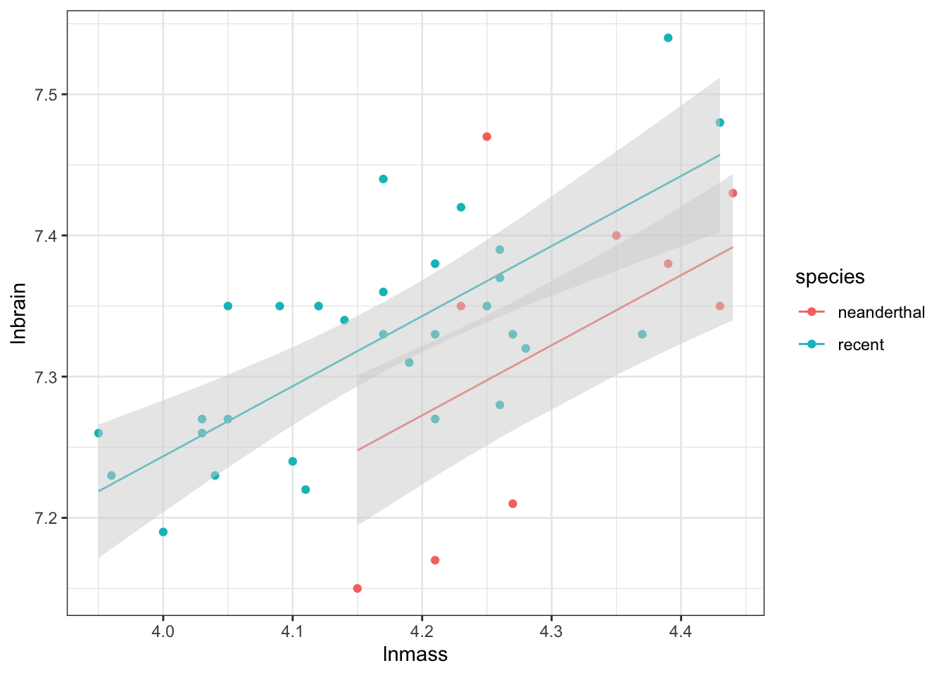
And there we have nice parallel lines with model predicted confidence intervals!
2.4 Examples
I’ve provided two data sets:
1) 18e4MoleRatLayabouts.csv looking at how caste and mass affect the energy mole rates expend.
18q11ExploitedLarvalFish.csvlooking at how status of a marine area - protected or not - influences the CV around age of maturity of a number of different fish (so, age is a predictor)
Using the following workflow, analyze these data sets.
# Load the data

# Perform a preliminary visualization

# Fit a model

# Test Assumptions and modify model if needed

# Evaluate results

# Post-hocs if you can

# Visualize results
3. Interacting Categorical Variables
Going with that previous intertidal example, if you really looked, it was a factorial design, with multiple treatments and conditions.
intertidal <- read.csv("./data/18e3IntertidalAlgae.csv")

ggplot(intertidal,
       mapping = aes(x = herbivores, y = sqrtarea,
                     fill = height)) +
  geom_boxplot()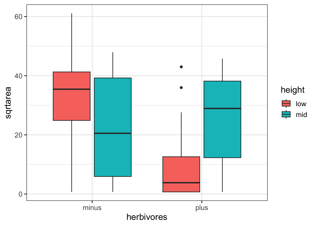
3.1 Fit and Assumption Evaluation
We fit factorial models using one of two different notations - both expand to the same thing
intertidal_lm <- lm(sqrtarea ~ herbivores + height + herbivores:height, data=intertidal)

intertidal_lm <- lm(sqrtarea ~ herbivores*height, data=intertidal)
Both mean the same thing as : is the interaction. * just means, expand all the interactions.
But, after that’s done…all of the assumption tests are the same. Try them out.
check_model(intertidal_lm)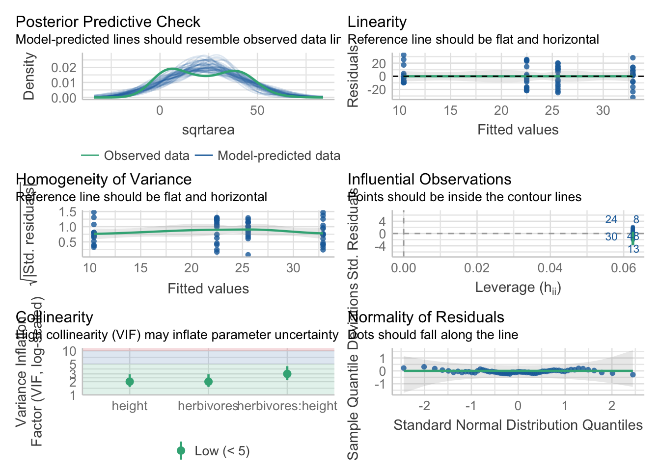
3.2 Post-Hocs
Post-hocs are a bit funnier. But not by much. As we have an interaction, let’s look at the simple effects. There are a few ways we can do this
emmeans(intertidal_lm, ~ herbivores + height) herbivores height emmean SE df lower.CL upper.CL
minus low 32.9 3.86 60 25.20 40.6
plus low 10.4 3.86 60 2.69 18.1
minus mid 22.5 3.86 60 14.77 30.2
plus mid 25.6 3.86 60 17.84 33.3
Confidence level used: 0.95 emmeans(intertidal_lm, ~ herbivores | height)height = low:
herbivores emmean SE df lower.CL upper.CL
minus 32.9 3.86 60 25.20 40.6
plus 10.4 3.86 60 2.69 18.1
height = mid:
herbivores emmean SE df lower.CL upper.CL
minus 22.5 3.86 60 14.77 30.2
plus 25.6 3.86 60 17.84 33.3
Confidence level used: 0.95 emmeans(intertidal_lm, ~ height | herbivores)herbivores = minus:
height emmean SE df lower.CL upper.CL
low 32.9 3.86 60 25.20 40.6
mid 22.5 3.86 60 14.77 30.2
herbivores = plus:
height emmean SE df lower.CL upper.CL
low 10.4 3.86 60 2.69 18.1
mid 25.6 3.86 60 17.84 33.3
Confidence level used: 0.95 Notice how each presents the information in a different way. The numbers are not different, they just show you information in different ways. The contrasts each reference grid implies do make s difference, though, in how p-value corrections for FWER is handled. Consider the first case.
emmeans(intertidal_lm, ~ herbivores + height) |>
  contrast(method = "pairwise")
contrast estimate SE df t.ratio p.value
minus low - plus low 22.51 5.45 60 4.128 0.0006
minus low - minus mid 10.43 5.45 60 1.913 0.2336
minus low - plus mid 7.36 5.45 60 1.350 0.5350
plus low - minus mid -12.08 5.45 60 -2.215 0.1307
plus low - plus mid -15.15 5.45 60 -2.778 0.0357
minus mid - plus mid -3.07 5.45 60 -0.563 0.9427
P value adjustment: tukey method for comparing a family of 4 estimates OK, cool. Every comparison is made. But what if we don’t want to do that? What if we just want to see if the herbivore effect differs by height?
emmeans(intertidal_lm, ~ herbivores | height) |>
  contrast(method = "pairwise")
height = low:
contrast estimate SE df t.ratio p.value
minus - plus 22.51 5.45 60 4.128 0.0001
height = mid:
contrast estimate SE df t.ratio p.value
minus - plus -3.07 5.45 60 -0.563 0.5758Notice that, because we’re only doing two contrasts, the correction is not as extreme. This method of contrasts might be more what you are interested in given your question. We can also see how this works visuall.
cont <- emmeans(intertidal_lm, ~ herbivores | height) |>
  contrast(method = "pairwise")

plot(cont) +
  geom_vline(xintercept = 0, color = "red", lty = 2)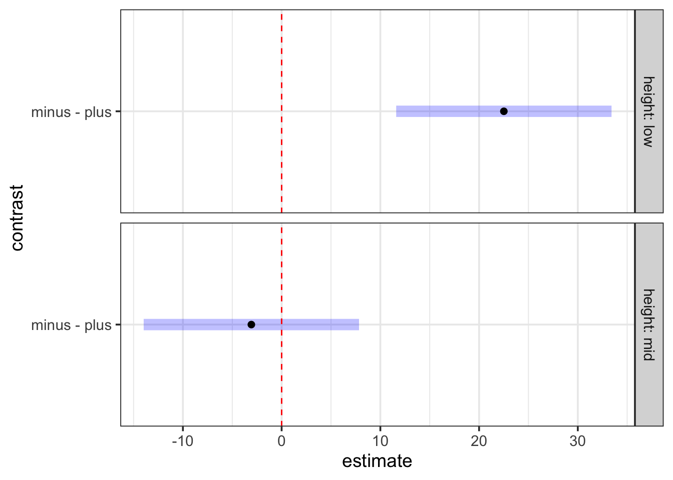
1.3 A Kelpy example
Let’s just jump right in with an example, as you should have all of this well in your bones by now. This was from a kelp, predator-diversity experiment I ran ages ago. Note, some things that you want to be factors might be loaded as
kelp <- read_csv("lab/data/kelp_pred_div_byrnesetal2006.csv")

## Check and correct for non-character
## variables - (TRIAL!)
## (this is some dplyr fun)
____________
_________


#Visualize
________(data = _____,
         aes(Treatment, Porp_Change, fill=Trial)) +
  geom______()

#fit
kelp_lm <- __(______ ~ ______ * _____, data=________)

#assumptions
performance::_______(__________)

# look at the model
broom::____________(__________)

# how well did we explain the data?
________(_____________)

#Pairwise Comparison of simple effects
emmeans(_______, specs = ~ __________ |___________) |>
  contrast(method = "________")
3.4 Replicated Regression and mixing Categorical and Continuous Variables
So…. the above was actually a replicated regression design. This is a design where you have continuous treatments, but you replicate at each treatment level. There are a few ways to deal with this. Note the column Predator_Diversity
Try this whole thing as a model with diversity as a continuous predictor an interaction by trial. What do you see?
Note - this is a great time to try out emmeans::emtrends().
Make a new column that is Predator_Diversity as a factor. Refit the factorial ANOVA with this as your treatment. Now try a pairwise test. What do you see? Visualize both. How do they give you different information? What would you conclude?
4. Interaction Effects in MLR
Let’s use the keeley fire severity plant richness data to see it Multiple Linear Regression with interaction effects action.
data(keeley)

ggpairs(keeley)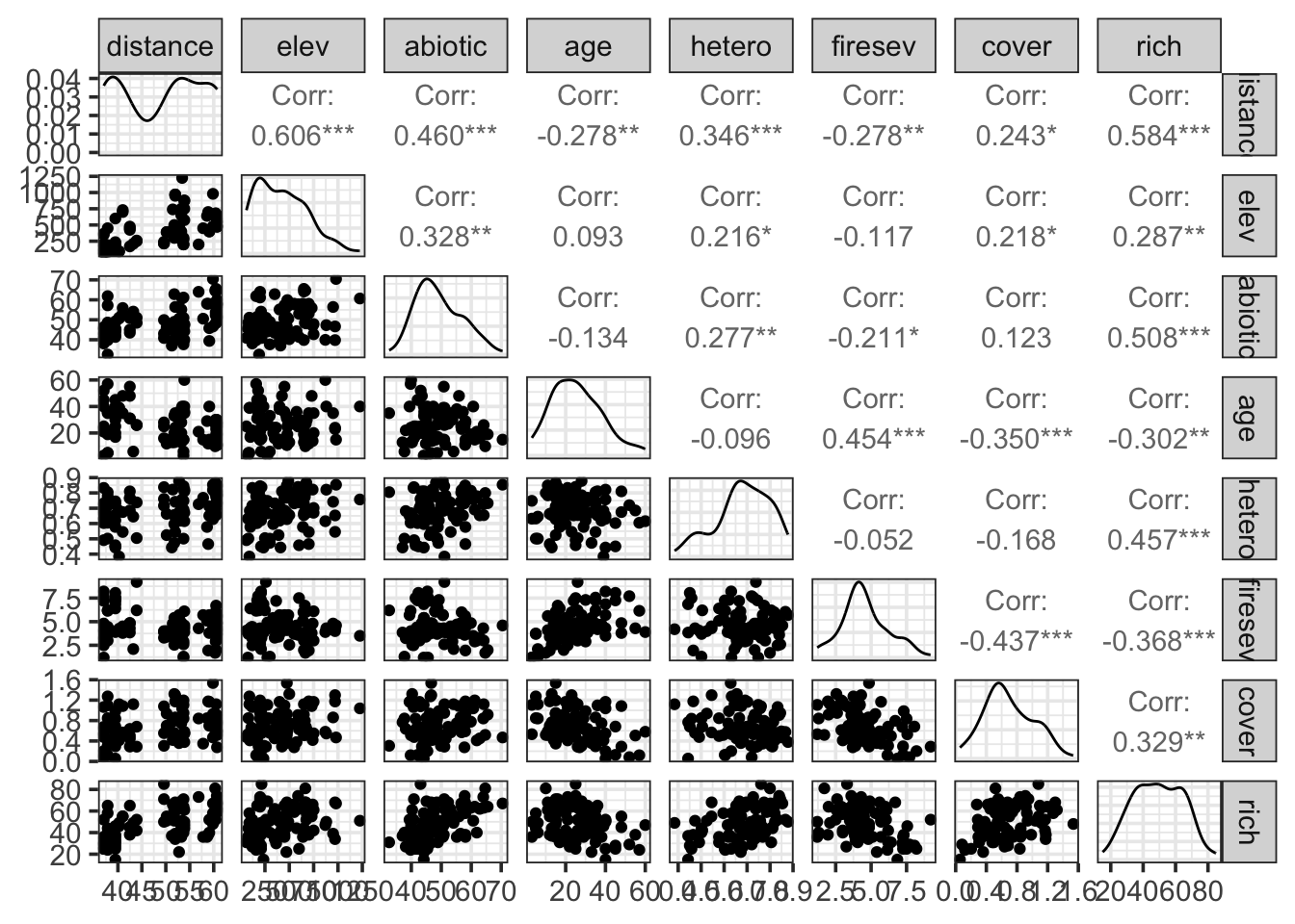
For our purposes, we’ll focus on fire severity and plot age as predictors of richness.
4.1 Explore and Model
What if there was an interaction here? One reasonable hypothesis is that fires affect stands of different ages differently. So, let’s look at richness as a function of age and fire severity. First, we’ll visualize, then fit a model.
ggplot(keeley,
       aes(x = age, y = rich, color = firesev)) +
  geom_point(size = 2) +
  scale_color_viridis_c(option = "B") +
  facet_wrap(~cut_number(firesev, 4))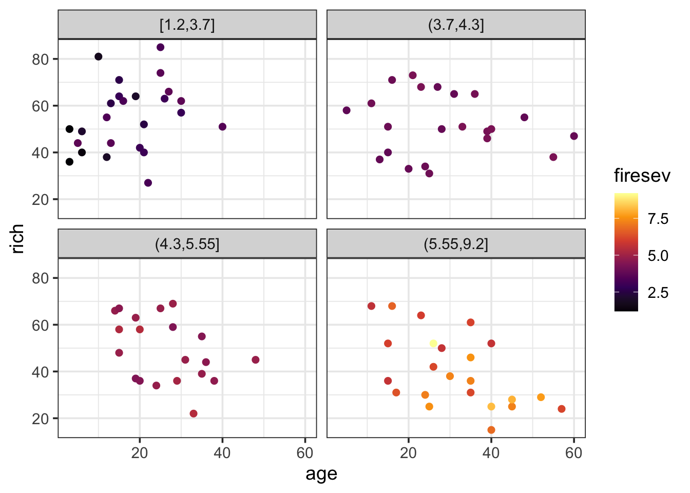
Huh. Kinda looks like age doesn’t have any effect until high fire severity.
keeley_mlr_int <- lm(rich ~ age * firesev, data=keeley)4.2 Assumptions
The assumptions here are the same as for MLR - normality of residuals, homoscedasticity, the relationship should not be driven by outliers alone, and, of course, lack of collinearity. Let’s explore the first few.
check_model(keeley_mlr_int)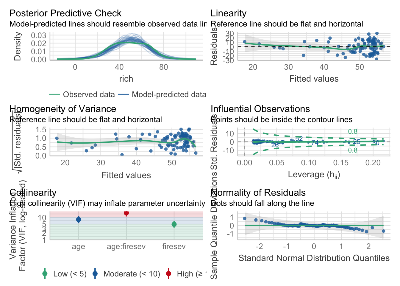
Also, excellent. Now, the vif…
vif(keeley_mlr_int)there are higher-order terms (interactions) in this model
consider setting type = 'predictor'; see ?vif age firesev age:firesev
7.967244 4.879394 15.800768 Oh hey! It tells us there’s a problem with interactions. I like performance’s solution even more.
check_collinearity(keeley_mlr_int)Model has interaction terms. VIFs might be inflated.
You may check multicollinearity among predictors of a model without
interaction terms.# Check for Multicollinearity
Low Correlation
Term VIF VIF 95% CI Increased SE Tolerance Tolerance 95% CI
firesev 4.88 [ 3.52, 6.98] 2.21 0.20 [0.14, 0.28]
Moderate Correlation
Term VIF VIF 95% CI Increased SE Tolerance Tolerance 95% CI
age 7.97 [ 5.62, 11.51] 2.82 0.13 [0.09, 0.18]
High Correlation
Term VIF VIF 95% CI Increased SE Tolerance Tolerance 95% CI
age:firesev 15.80 [10.95, 23.01] 3.98 0.06 [0.04, 0.09]Let’s look at the correlation between the predictors to see if there really is a problem.
keeley %>% select(firesev, age) %>%
  mutate(int = firesev*age) %>%
  cor()
firesev age int
firesev 1.0000000 0.4538654 0.7743624
age 0.4538654 1.0000000 0.8687952
int 0.7743624 0.8687952 1.0000000OK, the interaction is pretty highly correlated with age. But, well, again, not really a problem unless it is for the algorithm you are working with. We can instead look at the age-firesev correlation, which is only 0.45. We’re fine.
4.3 Centering?
Well, if we did want to worry about this - or were using an algorithm that choked - one way to break that correlation is to center our predictors before using them in the relationship. It changes the meaning of the coefficients, but, the model results are the same. Let’s try that here.
keeley <- keeley %>%
  mutate(firesev_c = firesev - mean(firesev),
         age_c = age - mean(age))

keeley_mlr_int_c <- lm(rich ~ age_c * firesev_c, data=keeley)

vif(keeley_mlr_int_c)
there are higher-order terms (interactions) in this model
consider setting type = 'predictor'; see ?vif age_c firesev_c age_c:firesev_c
1.261883 1.261126 1.005983 We see the vif is now small. Moreover…
keeley %>% select(firesev_c, age_c) %>%
  mutate(int = firesev_c*age_c) %>%
  cor()
firesev_c age_c int
firesev_c 1.00000000 0.45386536 -0.06336909
age_c 0.45386536 1.00000000 -0.06792114
int -0.06336909 -0.06792114 1.00000000Look at that correlation melt away. We’re still explaining variation in the same way. Let’s see how the coefficients differ.
coef(keeley_mlr_int)(Intercept) age firesev age:firesev
42.9352358 0.8268119 3.1056379 -0.2302444 coef(keeley_mlr_int_c) (Intercept) age_c firesev_c age_c:firesev_c
51.3790453 -0.2242540 -2.7809451 -0.2302444 So, in the no interaction model, the intercept is the richness when age and firesev are 0. The age and firesev effects are their effect when the other is 0, respectively. And the interaction is how they modify one another. Note that in the centered model, the interaction is the same. But, now the intercept is the richness at the average level of both predictors, and the additive predictors are the effects of each predictor at the average level of the other.
4.4 Evaluate
Given the lack of difference between the two models, we’re going to work with the original one. We’ve seen the coefficients and talked about their interpretation. The rest of the output can be interpreted as usual for a linear model.
tidy(keeley_mlr_int)# A tibble: 4 × 5
term estimate std.error statistic p.value
<chr> <dbl> <dbl> <dbl> <dbl>
1 (Intercept) 42.9 7.85 5.47 0.000000437
2 age 0.827 0.313 2.64 0.00981
3 firesev 3.11 1.86 1.67 0.0992
4 age:firesev -0.230 0.0641 -3.59 0.000548 Not that it doesn’t look like fire severity has an effect when age is 0. But what does age = 0 really mean? This is one reason by often the centered model is more interpretable.
So, how do we understand the interaction?
We can do things like calculate out the effect of one predictor at different levels of the other…
tibble(age = 0:10) %>%
  mutate(fire_effect = coef(keeley_mlr_int)[3] + coef(keeley_mlr_int)[4]*age)
# A tibble: 11 × 2
age fire_effect
<int> <dbl>
1 0 3.11
2 1 2.88
3 2 2.65
4 3 2.41
5 4 2.18
6 5 1.95
7 6 1.72
8 7 1.49
9 8 1.26
10 9 1.03
11 10 0.803But this can be unsatisfying, and we have to propogate error and - ECH. Why not try and create something more intuitive…
4.5 Visualize Results
Fundamentally, we have to create visualizations that look at different levels of both predictors somehow. There are a number of strategies.
4.5.1 Visreg
We can begin by looking at the effect of one variable at different levels of the other.
visreg(keeley_mlr_int, "age", "firesev", gg=TRUE)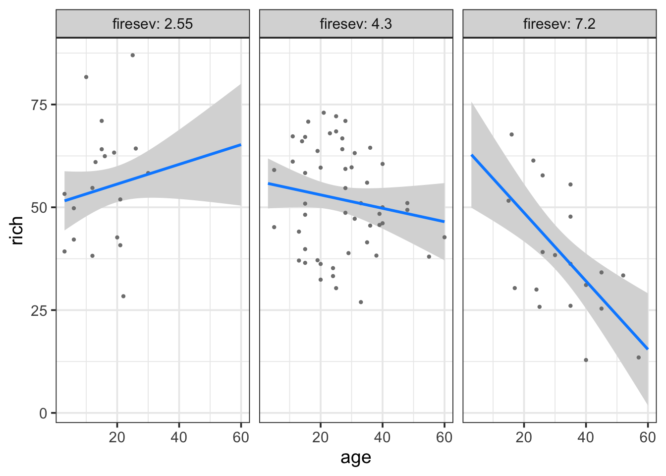
Here we see a plot where the points are adjusted for different levels of fireseverity - an even split between three levels - and then we see the resulting fit lines. We can of course reverse this, if we’re ore interested in the other effect.
visreg(keeley_mlr_int, "firesev", "age", gg=TRUE)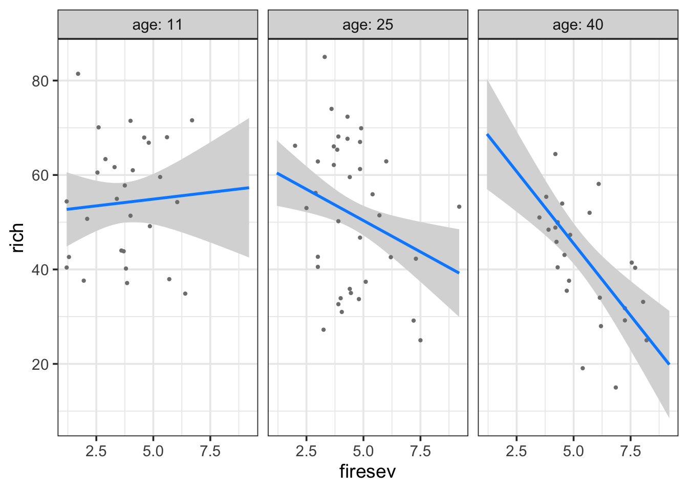
Both tell a compelling story of changing slopes that are easily understood. For example, in the later, fire has a stronger effect on older stands.
4.5.2 Fitted Model under Different Conditions
We might want to roll our own, however, and see the plot with different slices of the data. Fortunately, we can use the identical strategy as our MLR above - only now the slope changes. So, using the same strategy as above for making predicted data frames:
k_int_explore <- data_grid(keeley,
                               firesev = seq_range(firesev, 100),
                               age = seq_range(age, 4)) |>
  augment(keeley_mlr_int, newdata = _, interval = "confidence") |>
  rename(rich = .fitted)
Notice the lack of difference. We can now play with how we want to plot this. Here’s one, but you can come up with others easily.
ggplot(keeley,
       aes(x = firesev, y = rich, color = age)) +
  geom_point() +
  geom_line(data = k_int_explore, aes(group = age)) +
  geom_ribbon(data = k_int_explore, aes(ymin = .lower, ymax = .upper), alpha = 0.2, color = NA) +
  facet_wrap(~cut_interval(age,4)) +
  scale_color_viridis_c(option = "D")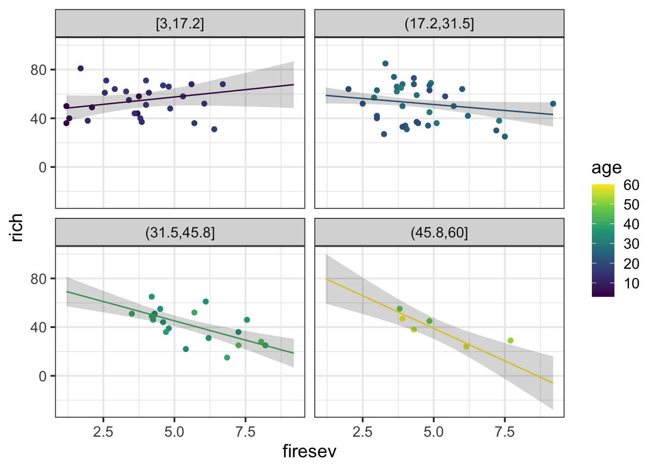
4.5.3 Surface Plot of Model
Finally, a surface plot can be very helpful - particularly under a condition of many interactions. To make a surface plot, we can look at the model and exract values at the intersection of multiple predictors and then visualize a grid where color or some other property reflects predicted values. It lets us see more nuance about an interaction. Let’s start with getting our surface values for a 100x100 grid of predictors.
keeley_surface <- data_grid(keeley,
                            age = seq_range(age, 100),
                            firesev = seq_range(firesev, 100)) |>
  augment(keeley_mlr_int, newdata = _) |>
  rename(rich = .fitted)
Now, we can plot this grid using geom_raster or geom_tile (raster will smooth things a bit).
ggplot(keeley_surface,
       aes(x = age, y = firesev, fill = rich)) +
  geom_raster() +
  scale_fill_viridis_c(option = "B")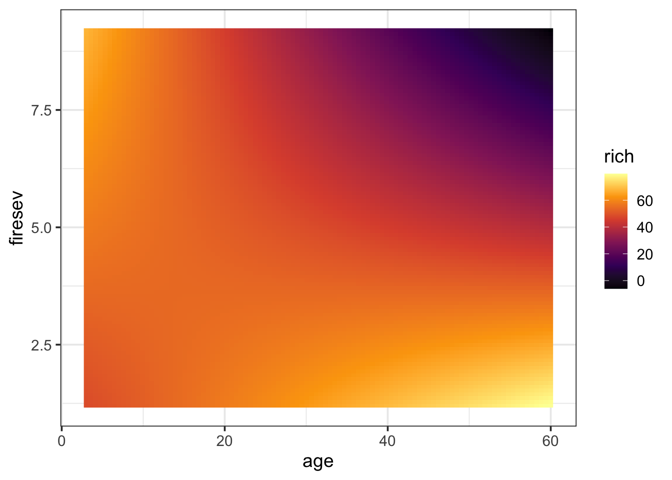
Now we can see the landscape more clearly. old stands with high fire severity have low richness. However, either youth or low fire severity means higher richness. This kind of technique can be great with higher order interactions. For example, you can facet by up to two variables (or more) to examine higher order interactions, etc.
Also note, if you want to be lazy, you can do this with visreg for two variables
visreg2d(keeley_mlr_int, "age", "firesev")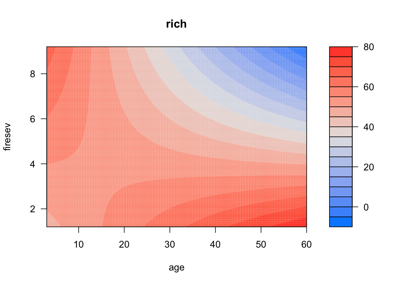
Last, what about a REAL surface? We can use plotly to help us here.
library(plotly)


surf_plotly <- plot_ly(x=~age, y=~firesev, z=~rich,
        type="scatter3d", mode="surface",
        data = keeley_surface, color = ~firesev)

surf_plotly
And if we want to add data points to it…
surf_plotly |>
  add_markers(data = keeley,
              x=~age, y=~firesev, z=~rich,
              color = I("black"))
4.6 Examples
OK, here are two datasets to work with. Choose one, and play around with possible interactions using ggplot. Then fit and evaluate a model!
planktonSummary.csvshowing plankton from Lake Biakal (thanks, Stephanie Hampton). Evluate how Chlorophyll (CHLFa) is affected by other predictors.Data on plant species richness in grazed salt marsh meadows in Finland. Meadows are grazed or ungrazed. see
?piecewiseSEM::meadowsto learn more. To load:
data(meadows, package = "piecewiseSEM")- If you are tired of biology, see
data(tips, package = "reshape")which looks at factors which might influence the tips given to one waiter over a few months. See?reshape:tips.
# Load the data

# Perform a preliminary visualization. Play with this and choose two predictors

# Fit a MLR model with an interaction

# Test Asssumptions and modify model if needed

# Evaluate results

# Visualize results