Making P-Values with Models

1. Linear Models

2. Generalized Linear Models & Likelihood

3. Mixed Models

Common Regression Test Statistics

• Are my coefficients 0?
  • Null Hypothesis: Coefficients are 0
  • Test Statistic: T distribution (normal distribution modified for low sample size)

• Does my model explain variability in the data?
  • Null Hypothesis: The ratio of variability from your predictors versus noise is 1
  • Test Statistic: F distribution (describes ratio of two variances)

T-Distributions are What You'd Expect Sampling a Standard Normal Population with a Small Sample Size

• t = mean/SE, DF = n-1
• It assumes a normal population with mean of 0 and SD of 1

Assessing the Slope with a T-Test

$$\Large t_{b} = \frac{b - \beta_{0}}{SE_{b}}$$

DF=n-2

$H_0: \beta_{0} = 0$, but we can test other hypotheses

Slope of Puffer Relationship (DF = 1 for Parameter Tests)

p is very small here so...
We reject the hypothesis of no slope for resemblance, but fail to reject it for the intercept.

So, what can we say in a null hypothesis testing framework?

Does my model explain variability in the data?

Ho = The model predicts no variation in the data.

Ha = The model predicts variation in the data.

To evaluate these hypotheses, we need to have a measure of variation explained by data versus error - the sums of squares!

This is an Analysis of Variance..... ANOVA! $$SS_{Total} = SS_{Regression} + SS_{Error}$$

Sums of Squares of Error, Visually

Sums of Squares of Regression, Visually

Distance from $\hat{y}$ to $\bar{y}$

Components of the Total Sums of Squares

$SS_{R} = \sum(\hat{Y_{i}} - \bar{Y})^{2}$, df=1

$SS_{E} = \sum(Y_{i} - \hat{Y}_{i})^2$, df=n-2

To compare them, we need to correct for different DF. This is the Mean Square.

MS=SS/DF

e.g, $MS_{E} = \frac{SS_{E}}{n-2}$

The F Distribution and Ratios of Variances

$F = \frac{MS_{R}}{MS_{E}}$ with DF=1,n-2

F-Test and Pufferfish

We reject the null hypothesis that resemblance does not explain variability in predator approaches

Testing the Coefficients

• F-Tests evaluate whether elements of the model contribute to variability in the data
  • Are modeled predictors just noise?
  • What's the difference between a model with only an intercept and an intercept and slope?

• T-tests evaluate whether coefficients are different from 0

• Often, F and T agree - but not always

  • T can be more sensitive with multiple predictors

What About Models with Categorical Variables?

• T-tests for Coefficients with Treatment Contrasts

• F Tests for Variability Explained by Including Categorical Predictor

  • ANOVA

• More T-Tests for Posthoc Evaluation

What Explains This Data? Same as Regression (because it's all a linear model)

Variability due to Model (between groups)

Variability due to Error (Within Groups)

F-Test to Compare

$SS_{Total} = SS_{Model} + SS_{Error}$

(Classic ANOVA: $SS_{Total} = SS_{Between} + SS_{Within}$)

Yes, these are the same!

F-Test to Compare

$SS_{Model} = \sum_{i}\sum_{j}(\bar{Y_{i}} - \bar{Y})^{2}$, df=k-1

$SS_{Error} = \sum_{i}\sum_{j}(Y_{ij} - \bar{Y_{i}})^2$, df=n-k

To compare them, we need to correct for different DF. This is the Mean Square.

MS = SS/DF, e.g, $MS_{W} = \frac{SS_{W}}{n-k}$

ANOVA

We have strong confidence that we can reject the null hypothesis

This Works the Same for Multiple Categorical

TreatmentHo: $\mu_{i1} = \mu{i2} = \mu{i3} = ...$

Block Ho: $\mu_{j1} = \mu{j2} = \mu{j3} = ...$

i.e., The variance due to each treatment type is no different than noise

We Decompose Sums of Squares for Multiple Predictors

$SS_{Total} = SS_{A} + SS_{B} + SS_{Error}$

• Factors are Orthogonal and Balanced, so, Model SS can be split
  • F-Test using Mean Squares as Before

What About Unbalanced Data or Mixing in Continuous Predictors?

• Let's Assume Y ~ A + B where A is categorical and B is continuous

• F-Tests are really model comparisons

• The SS for A is the Residual SS of Y ~ A + B - Residual SS of Y ~ B

  • This type of SS is called marginal SS or type II SS

• Proceed as normal

• This also works for interactions, where interactions are all tested including additive or lower-level interaction components

  • e.g., SS for AB is RSS for A+B+AB - RSS for A+B

Warning for Working with SAS Product Users (e.g., JMP)

• You will sometimes see Type III which is sometimes nonsensical
  • e.g., SS for A is RSS for A+B+AB - RSS for B+AB

• Always question the default settings!

Post-Hoc Comparisons of Groups

• Only compare groups if you reject a Null Hypothesis via F-Test
  • Otherwise, any results are spurious
  • This is why they are called post-hocs

• We've been here before with SEs and CIs

• In truth, we are using T-tests

• BUT - we now correct p-values for Family-Wise Error (if at all)

Making P-Values with Models

1. Linear Models

2. Generalized Linear Models & Likelihood

3. Mixed Models

To Get There to Testing, We Need To Understand Likelihood and Deviance

.center[

Likelihood Defined

$$\Large L(H | D) = p(D | H)$$

Where the D is the data and H is the hypothesis (model) including a both a data generating process with some choice of parameters (often called $\theta$). The error generating process is inherent in the choice of probability distribution used for calculation.

MLE for Multiple Data Points

Let's say this is our data:

 [1]  3.37697212  3.30154837  1.90197683  1.86959410  0.20346568  3.72057350
 [7]  3.93912102  2.77062225  4.75913135  3.11736679  2.14687718  3.90925918
[13]  4.19637296  2.62841610  2.87673977  4.80004312  4.70399588 -0.03876461
[19]  0.71102505  3.05830349

We know that the data comes from a normal population with a $\sigma$ of 1.... but we want to get the MLE of the mean.

$p(D|\theta) = \prod p(D_i|\theta)$

    = $\prod dnorm(D_i, \mu, \sigma = 1)$

Likelihood At Different Choices of Mean, Visually

The Likelihood Surface

MLE = 2.896

The Log-Likelihood Surface

We use Log-Likelihood as it is not subject to rounding error, and approximately $\chi^2$ distributed.

The $\chi^2$ Distribution

• Distribution of sums of squares of k data points drawn from N(0,1)

• k = Degrees of Freedom

• Measures goodness of fit

• A large probability density indicates a match between the squared difference of an observation and expectation

The $\chi^2$ Distribution, Visually

Hey, Look, it's the Standard Error!

The 68% CI of a $\chi^2$ distribution is 0.49, so....

Hey, Look, it's the 95% CI!

The 95% CI of a $\chi^2$ distribution is 1.92, so....

The Deviance: -2 * Log-Likelihood

• Measure of fit. Smaller deviance = closer to perfect fit
• We are minimizing now, just like minimizing sums of squares
• Point deviance residuals have meaning
• Point deviance of linear regression = mean square error!

Putting MLE Into Practice with Pufferfish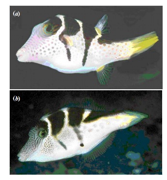

This is our fit relationship

Likelihood Function for Linear Regression

Likelihood Function for Linear Regression: What it Means

$$L(\theta | Data) = \prod_{i=1}^n \mathcal{N}(Visits_i\; |\; \beta_{0} + \beta_{1} Resemblance_i, \sigma)$$

where $\beta_{0}, \beta_{1}, \sigma$ are elements of $\theta$

The Log-Likelihood Surface from Grid Sampling

Let's Look at Profiles to get CIs

Evaluate Coefficients

Test Statistic is a Wald Z-Test Assuming a well behaved quadratic Confidence Interval

Can Compare p(data | H) for alternate Parameter Values - and it could be 0!

Compare $p(D|\theta_{1})$ versus $p(D|\theta_{2})$

Likelihood Ratios

$$\LARGE G = \frac{L(H_1 | D)}{L(H_2 | D)}$$

• G is the ratio of Maximum Likelihoods from each model

• Used to compare goodness of fit of different models/hypotheses

• Most often, $\theta$ = MLE versus $\theta$ = 0

• $-2 log(G)$ is $\chi^2$ distributed

Likelihood Ratio Test

• A new test statistic: $D = -2 log(G)$

• $= 2 [Log(L(H_2 | D)) - Log(L(H_1 | D))]$

• We then scale by dispersion parameter (e.g., variance, etc.)

• It's $\chi^2$ distributed!

  • DF = Difference in # of Parameters

• If $H_1$ is the Null Model, we have support for our alternate model

Likelihood Ratio Test for Regression

• We compare our slope + intercept to a model fit with only an intercept!

• Note, models must have the SAME response variable

int_only <- glm(predators ~ 1, data = puffer)

• We then use Analysis of Deviance (ANODEV)

Our First ANODEV

Analysis of Deviance Table
Model 1: predators ~ 1
Model 2: predators ~ resemblance
  Resid. Df Resid. Dev Df Deviance  Pr(>Chi)    
1        19     422.95                          
2        18     167.80  1   255.15 1.679e-07 ***
---
Signif. codes:  0 '***' 0.001 '**' 0.01 '*' 0.05 '.' 0.1 ' ' 1

Note, uses Difference in Deviance / Dispersion where Dispersion = Variance as LRT

Or, R has Tools to Automate Doing This Piece by Piece

Analysis of Deviance Table (Type II tests)
Response: predators
            LR Chisq Df Pr(>Chisq)    
resemblance   27.371  1  1.679e-07 ***
---
Signif. codes:  0 '***' 0.001 '**' 0.01 '*' 0.05 '.' 0.1 ' ' 1

Here, LRT = Difference in Deviance / Dispersion where Dispersion = Variance

Making P-Values with Models

1. Linear Models

2. Generalized Linear Models & Likelihood

3. Mixed Models

Let's take this to the beach with Tide Height: RIKZ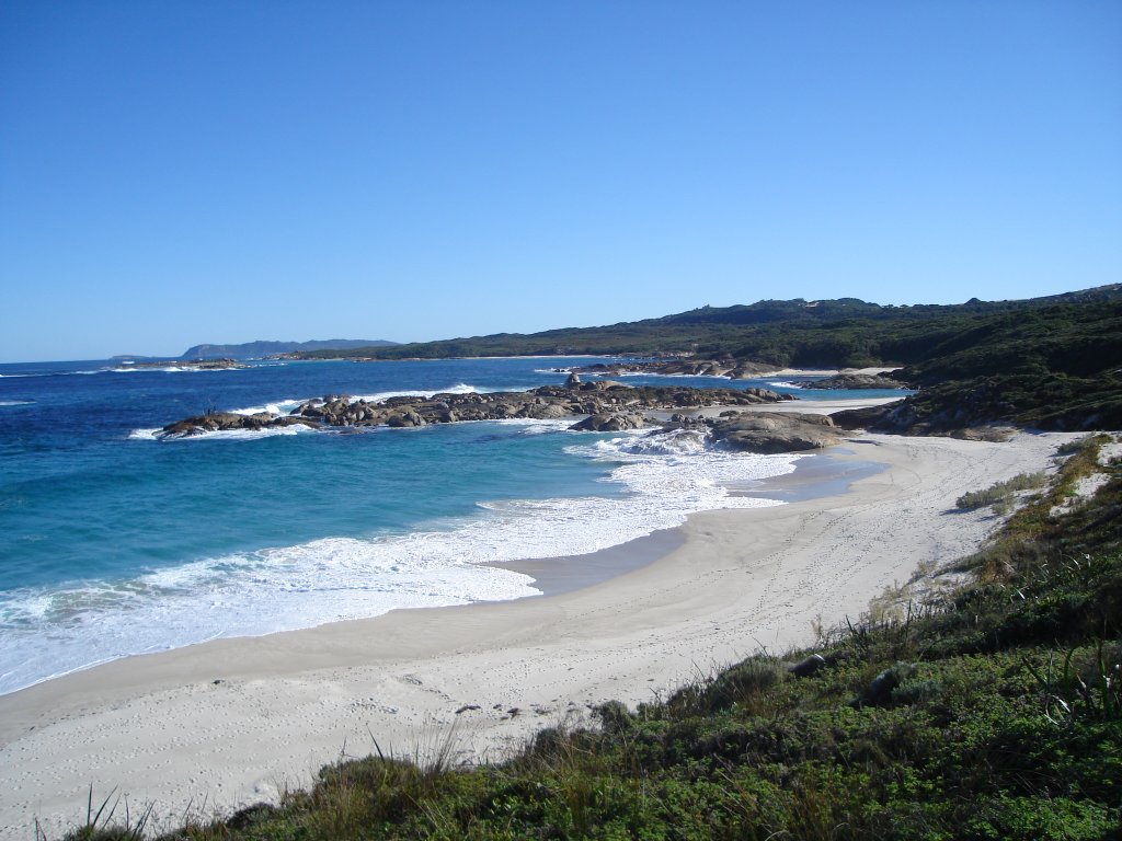

How is Tidal Height of Measurement Associated With Species Richness?

Approaches to approximating DF

• Satterthwaite approximation - Based on sample sizes and variances within groups

  • lmerTest (which is kinda broken at the moment)

• Kenward-Roger’s approximation.

  • Based on estimate of variance-covariance matrix of fixed effects and a scaling factor
  • More conservative - in car::Anova() and pbkrtest

Compare!

Baseline - only for balanced LMMs!

Analysis of Variance Table
    npar Sum Sq Mean Sq F value
NAP    1 10.467  10.467  63.356

Satterwaith

Type III Analysis of Variance Table with Satterthwaite's method
    Sum Sq Mean Sq NumDF  DenDF F value    Pr(>F)    
NAP 10.467  10.467     1 37.203  63.356 1.495e-09 ***
---
Signif. codes:  0 '***' 0.001 '**' 0.01 '*' 0.05 '.' 0.1 ' ' 1

Kenward-Roger

Analysis of Deviance Table (Type II Wald F tests with Kenward-Roger df)
Response: log_richness
         F Df Df.res    Pr(>F)    
NAP 62.154  1 37.203 1.877e-09 ***
---
Signif. codes:  0 '***' 0.001 '**' 0.01 '*' 0.05 '.' 0.1 ' ' 1

The Smaller Questions and Answers

1. With REML (for lmms), we often are conservative in our estimation of fixed effects. Should we use it?
   • use ML for FE tests if using Chisq

1. Should we use Chi-Square?
   • for GLMMs, yes.
   • Can be unreliable in some scenarios.
   • Use F tests for lmms

F and Chisq

F-test

# A tibble: 1 × 5
  term  statistic    df Df.res       p.value
  <chr>     <dbl> <dbl>  <dbl>         <dbl>
1 NAP        62.2     1   37.2 0.00000000188

LR Chisq

# A tibble: 1 × 4
  term  statistic    df  p.value
  <chr>     <dbl> <dbl>    <dbl>
1 NAP        63.4     1 1.72e-15

LR Chisq where REML = FALSE

# A tibble: 1 × 4
  term  statistic    df  p.value
  <chr>     <dbl> <dbl>    <dbl>
1 NAP        65.6     1 5.54e-16

What about Random Effects

• For LMMs, make sure you have fit with REML = TRUE

• One school of thought is to leave them in place

  • Your RE structure should be determined by sampling design
  • Do you know enough to change your RE structure?

• But sometimes you need to test!
  • Can sequentially drop RE effects with lmerTest::ranova()
  • Can simulate models with 0 variance in RE with rlrsim, but gets tricky

RANOVA

ranova(rikz_varint)

ANOVA-like table for random-effects: Single term deletions
Model:
log_richness ~ NAP + (1 | Beach)
            npar  logLik    AIC    LRT Df Pr(>Chisq)    
<none>         4 -32.588 73.175                         
(1 | Beach)    3 -38.230 82.460 11.285  1  0.0007815 ***
---
Signif. codes:  0 '***' 0.001 '**' 0.01 '*' 0.05 '.' 0.1 ' ' 1

Testing Mixed Models

1. Yes you can!

2. Some of the fun issues of denominator DF raise their heads

3. Keep up to date on the literature/FAQ when you are using them!