class: center, middle # So Many Variables: Multiple Linear Regression and Variable Selection  --- class: center, middle # Etherpad <br><br> <center><h3>https://etherpad.wikimedia.org/p/607-mlr-2020 </h3></center> --- # So many variables. 1. Multiple linear regression review 2. Multiple linear regression with interactions 3. Visualizaing MLR 4. The problem of what variables to choose: muti-model inference --- # Previously On Multiple Regression and the General Linear Model! .middle[.center[ 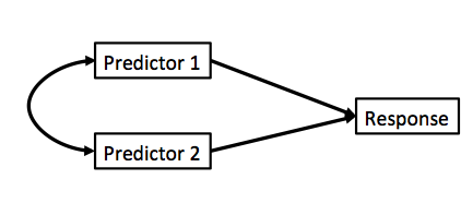 ] With multiple regression, we estimate the effect of one variable as if we were controlling for the other, given the covariance between predictors. ] --- background-image:url(images/23/fires.jpg) background-size:contain background-position:center class: bottom, inverse ### Five year study of wildfires & recovery in Southern California shurblands in 1993. 90 plots (20 x 50m) (data from Jon Keeley et al.) --- # What causes species richness? - Distance from fire patch - Elevation - Abiotic index - Patch age - Patch heterogeneity - Severity of last fire - Plant cover --- # Our Model `$$Richness_i =\beta_{0} + \beta_{1} cover_i +\beta_{2} firesev_i + \beta_{3}hetero_i +\epsilon_i$$` -- ```r klm <- lm(rich ~ cover + firesev + hetero, data=keeley) ``` --- # Evaluating If Multicollinearity is a Problem # Checking for Multicollinearity: Variance Inflation Factor `$$VIF_1 = \frac{1}{1-R^2_{1}}$$` ```r vif(klm) ``` ``` cover firesev hetero 1.294950 1.261695 1.050381 ``` --- # Other Diagnostics as Usual! <img src="mlr_int_files/figure-html/klm_diag-1.png" style="display: block; margin: auto;" /> --- # Modeled Results | | Estimate| Std. Error| t value| Pr(>&#124;t&#124;)| |:-----------|--------:|----------:|-------:|------------------:| |(Intercept) | 1.68| 10.67| 0.16| 0.88| |cover | 15.56| 4.49| 3.47| 0.00| |firesev | -1.82| 0.85| -2.14| 0.04| |hetero | 65.99| 11.17| 5.91| 0.00| - Coefficients are the change in units of y per change in 1 unit of X - Intercept is value of y when all variables are 0 --- # Comparing Coefficients on the Same Scale If we want to get Partial Correlation Coefficients, we can z-transform all predictors or use this formula: `$$r_{xy} = b_{xy}\frac{sd_{x}}{sd_{y}}$$` ``` cover firesev hetero 0.3267325 -0.1987243 0.5016017 ``` Now, `\(\beta\)`s are change in SD of Y per change in 1 SD of X --- # Viz is an art <img src="mlr_int_files/figure-html/klm_visreg-1.png" style="display: block; margin: auto;" /> --- # So many variables. 1. Multiple linear regression review 2. .red[Multiple linear regression with interactions] 3. Visualizaing MLR 4. The problem of what variables to choose: muti-model inference --- # Problem: What if Continuous Predictors are Not Additive? <img src="mlr_int_files/figure-html/keeley_int_plot3d-1.png" style="display: block; margin: auto;" /> --- # Problem: What if Continuous Predictors are Not Additive? <img src="mlr_int_files/figure-html/keeley_int_plot-1.png" style="display: block; margin: auto;" /> --- # Problem: What if Continuous Predictors are Not Additive? <img src="mlr_int_files/figure-html/keeley_int_plot2-1.png" style="display: block; margin: auto;" /> --- # Model For Age Interacting with Elevation to Influence Fire Severity `$$y_i = \beta_0 + \beta_{1}x_{1i} + \beta_{2}x_{2i}+ \beta_{3}x_{1i}x_{2i} + \epsilon_{i}$$` - Interaction is product of X1 and X2 - Can be as many interactions as you'd like - Honestly, you can do whatever feature engineering you want to make complex combinations of predictors! - But, multiplication is common -- Code just like factorial models! ```r keeley_lm_int <- lm(firesev ~ age*elev, data=keeley) ``` --- # A Problem: Interactions are Collinear with Predictors `$$VIF_1 = \frac{1}{1-R^2_{1}}$$` ```r vif(keeley_lm_int) ``` ``` age elev age:elev 3.200054 5.517494 8.287104 ``` -- This isn't that bad. But it can be. -- Often, interactions or nonlinear derived predictors are collinear with one or more of their predictors. -- To remove, this, we can **center** predictors - i.e., `\(X_i - mean(X)\)` --- # Interpretation of Centered Coefficients `$$\huge X_i - \bar{X}$$` - Additive coefficients are the effect of a predictor at the mean value of the other predictors -- - Intercepts are at the mean value of all predictors -- - This is good practice for regression models in general when 0 is meaningless for predictors -- - Also, relationships can become sharply nonlinear at 0, and you likely aren't modeling that correctly -- - Visualization will keep you from getting confused! --- # Interactions, VIF, and Centering `$$y = \beta_0 + \beta_{1}(x_{1}-\bar{x_{1}}) + \beta_{2}(x_{2}-\bar{x_{2}})+ \beta_{3}(x_{1}-\bar{x_{1}})(x_{2}-\bar{x_{2}})$$` -- Woof. That looks ugly. But, read it. It is not as complex as you think. -- Variance Inflation Factors for Centered Model: ``` age_c elev_c age_c:elev_c 1.016721 1.041830 1.037929 ``` --- # F-Tests to Evaluate Model What type of Sums of Squares?? -- | | Sum Sq| Df| F value| Pr(>F)| |:---------|----------:|--:|---------:|---------:| |age | 52.963196| 1| 27.709228| 0.0000010| |elev | 6.253129| 1| 3.271505| 0.0739877| |age:elev | 22.304523| 1| 11.669256| 0.0009722| |Residuals | 164.379710| 86| | | --- # Coefficients (non-centered model)! | | Estimate| Std. Error| t value| Pr(>&#124;t&#124;)| |:-----------|----------:|----------:|---------:|------------------:| |(Intercept) | 1.8132153| 0.6156070| 2.945411| 0.0041484| |age | 0.1206292| 0.0208618| 5.782298| 0.0000001| |elev | 0.0030852| 0.0013329| 2.314588| 0.0230186| |age:elev | -0.0001472| 0.0000431| -3.416029| 0.0009722| R² = 0.3235187 -- - Note that additive coefficients signify the effect of one predictor **in the absence of all others.** - Intercept is value of Y when all coefficients are 0 --- # Centered Coefficients! | | Estimate| Std. Error| t value| Pr(>&#124;t&#124;)| |:------------|----------:|----------:|---------:|------------------:| |(Intercept) | 4.6091266| 0.1463029| 31.503991| 0.0000000| |age_c | 0.0581123| 0.0117591| 4.941901| 0.0000038| |elev_c | -0.0006786| 0.0005792| -1.171587| 0.2445985| |age_c:elev_c | -0.0001472| 0.0000431| -3.416029| 0.0009722| R² = 0.3235187 -- - Note that additive coefficients signify the effect of one predictor **at the average level of all others.** - Intercept is value of Y at the **average level** of all predictors. --- # So many variables. 1. Multiple linear regression review 2. Multiple linear regression with interactions 3. .red[Visualizaing MLR] 4. The problem of what variables to choose: muti-model inference --- # Interpretation - What the heck does an interaction effect mean? -- - We can look at the effect of one variable at different levels of the other -- - We can look at a surface -- - We can construct *counterfactual* plots showing how changing both variables influences our outcome --- # Age at Different Levels of Elevation <img src="mlr_int_files/figure-html/int_visreg-1.png" style="display: block; margin: auto;" /> --- # Elevation at Different Levels of Age <img src="mlr_int_files/figure-html/int_visreg_2-1.png" style="display: block; margin: auto;" /> --- # Surfaces and Other 3d Objects <img src="mlr_int_files/figure-html/surf_int-1.png" style="display: block; margin: auto;" /> --- # Or all in one plot <img src="mlr_int_files/figure-html/keeley_int_pred-1.png" style="display: block; margin: auto;" /> --- # Without Data and Including CIs <img src="mlr_int_files/figure-html/keeley_int_pred_nodata-1.png" style="display: block; margin: auto;" /> --- # A Heatmap Approach <img src="mlr_int_files/figure-html/int_heatmap-1.png" style="display: block; margin: auto;" /> --- # You know know all the models - Interaction effects or other nonlinearities are often one of the most useful and yet hardest to grok parts of building models - BUT, if you can learn *how to understand* interactions in your model, you've reached the upper echelons - BUT, beware. Not every model needs an interaction - start with the fundamentals of theory and biology first --- class:middle, center  --- # So many variables. 1. Multiple linear regression review 2. Multiple linear regression with interactions 3. Visualizaing MLR 4. .red[The problem of what variables to choose: muti-model inference] --- # So.... How do you Choose What Variables to Include? 7 models alone with 1 term each 127 possible **without** interactions. #  --- class: center, middle ##Hint: The real answer is to think about biology - it's coming - but sometimes, you are doing pure exploration, so... --- # A Quantitative Measure of Relative Support `$$w_{i} = \frac{e^{-\Delta_{i}/2 }}{\displaystyle \sum^R_{r=1} e^{-\Delta_{i}/2 }}$$` Where `\(w_{i}\)` is the relative supporfor model i compared to other models in the set being considered. Model weights summed together = 1 --- # Let's Begin with a Full Model ```r keeley_full <- lm(rich ~ elev + abiotic + hetero + distance + firesev + age + cover, data = keeley) ``` We use this model as a jumping off point, and construct a series of nested models with subsets of the variables. Evaluate using AICc Weights! --- # Sometimes, You Can Use a Models broken down by CLASSES of Predictors ```r keeley_soil_fire <- lm(rich ~ elev + abiotic + hetero + distance + firesev, data = keeley) keeley_plant_fire <- lm(rich ~ distance + firesev + age + cover, data = keeley) keeley_soil_plant <- lm(rich ~ elev + abiotic + hetero + age + cover, data = keeley) ``` --- # One Factor Models .middle[ ```r keeley_soil <- lm(rich ~ elev + abiotic + hetero, data = keeley) keeley_fire <- lm(rich ~ distance + firesev, data = keeley) keeley_plant <- lm(rich ~ age + cover, data = keeley) ``` ] --- # Null Model .middle[ ```r keeley_null <- lm(rich ~ 1, data = keeley) ``` ] --- # Now Compare Models Weights | |Modnames | K| AICc| Delta_AICc| ModelLik| AICcWt| LL| |:--|:----------|--:|-------:|----------:|--------:|------:|--------:| |1 |full | 9| 688.162| 0.000| 1.000| 0.888| -333.956| |3 |soil_fire | 7| 692.554| 4.392| 0.111| 0.099| -338.594| |4 |soil_plant | 7| 696.569| 8.406| 0.015| 0.013| -340.601| |7 |fire | 4| 707.493| 19.331| 0.000| 0.000| -349.511| |2 |plant_fire | 6| 709.688| 21.526| 0.000| 0.000| -348.338| |5 |soil | 5| 711.726| 23.564| 0.000| 0.000| -350.506| |6 |plant | 4| 737.163| 49.001| 0.000| 0.000| -364.346| |8 |null | 2| 747.254| 59.092| 0.000| 0.000| -371.558| --- class:center, middle ## So, I have some sense of good models? What now? --- class: center, middle  --- # Variable Weights How to I evaluate the importance of a variable? -- Variable Weight = sum of all weights of all models including a variable. Relative support for inclusion of parameter in models. -- ``` Importance values of 'firesev': w+ (models including parameter): 0.99 w- (models excluding parameter): 0.01 ``` -- But what about the estimand and its precision? --- background-color: black class: center, middle  --- # We can Use Model Averaged Parameters `$$\hat{\bar{\beta}} = \frac{\sum w_{i}\hat\beta_{i}}{\sum{w_i}}$$` `$$var(\hat{\bar{\beta}}) = \left [ w_{i} \sqrt{var(\hat\beta_{i}) + (\hat\beta_{i}-\hat{\bar{\beta_{i}}})^2} \right ]^2$$` Buckland et al. 1997 --- # Model Averaged Parameters ```r modavgShrink(modelList, parm="firesev", modnames=names(modelList)) ``` ``` Multimodel inference on "firesev" based on AICc AICc table used to obtain model-averaged estimate with shrinkage: K AICc Delta_AICc AICcWt Estimate SE full 9 688.16 0.00 0.89 -1.02 0.80 plant_fire 6 709.69 21.53 0.00 -1.39 0.92 soil_fire 7 692.55 4.39 0.10 -1.89 0.73 soil_plant 7 696.57 8.41 0.01 0.00 0.00 soil 5 711.73 23.56 0.00 0.00 0.00 plant 4 737.16 49.00 0.00 0.00 0.00 fire 4 707.49 19.33 0.00 -2.03 0.80 null 2 747.25 59.09 0.00 0.00 0.00 Model-averaged estimate with shrinkage: -1.09 Unconditional SE: 0.84 95% Unconditional confidence interval: -2.74, 0.56 ``` --- class:center, middle background-color: black  --- # Best to Use Model Averaged Predictions ```r newData <- data.frame(distance = 50, elev = 400, abiotic = 48, age = 2, hetero = 0.5, firesev = 10, cover=0.4) ``` ``` Model-averaged predictions on the response scale based on entire model set and 95% confidence interval: mod.avg.pred uncond.se lower.CL upper.CL 1 31.666 6.136 19.64 43.692 ``` --- # Death to single models! - While sometimes the model you should use is clear, more often it is *not* -- - Further, you made those models for a reason: you suspect those terms are important -- - Better to look at coefficients across models -- - For actual predictions, ensemble predictions provide real uncertainty --- # What about IC Analyses in Bayes? .center[.middle[  ]] --- # Bayesian MMI - We can calculate an IC and Model Weight using LOOIC or WAIC - We can get weighted parameter estimates by sampling from the chains of different models in proportion to their IC weight - We can get MMI predictions by doing the same with predictions! --- # Final Notes on Many Models - If you can, don't do this. Start by building models and working up. We will talk about this soon. -- - BUT, if you are exploring model space, IC analyses aid in model selection. One must still evaluate parameters and parameter error. -- - Your inferences are constrained solely to the range of models you consider. You may have missed the ’best’ model for prediction. -- - Remember, this is ALL ABOUT PREDICTION -- - All inferences <span>**MUST**</span> be based on <span>*a* priori</span> models. Post-hoc model dredging could result in an erroneous ’best’ model suited to your unique data set. -- - Ensemble predictions are a powerful practice to show true uncertainty