Taking Least Squares From the Ordinary to the General(ized)

This is What you All Fear…
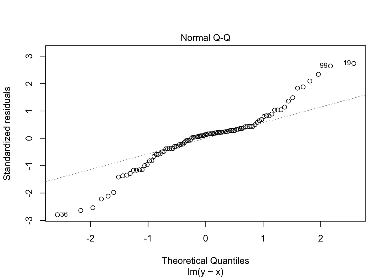
What do we do here?
Or, oh no!…
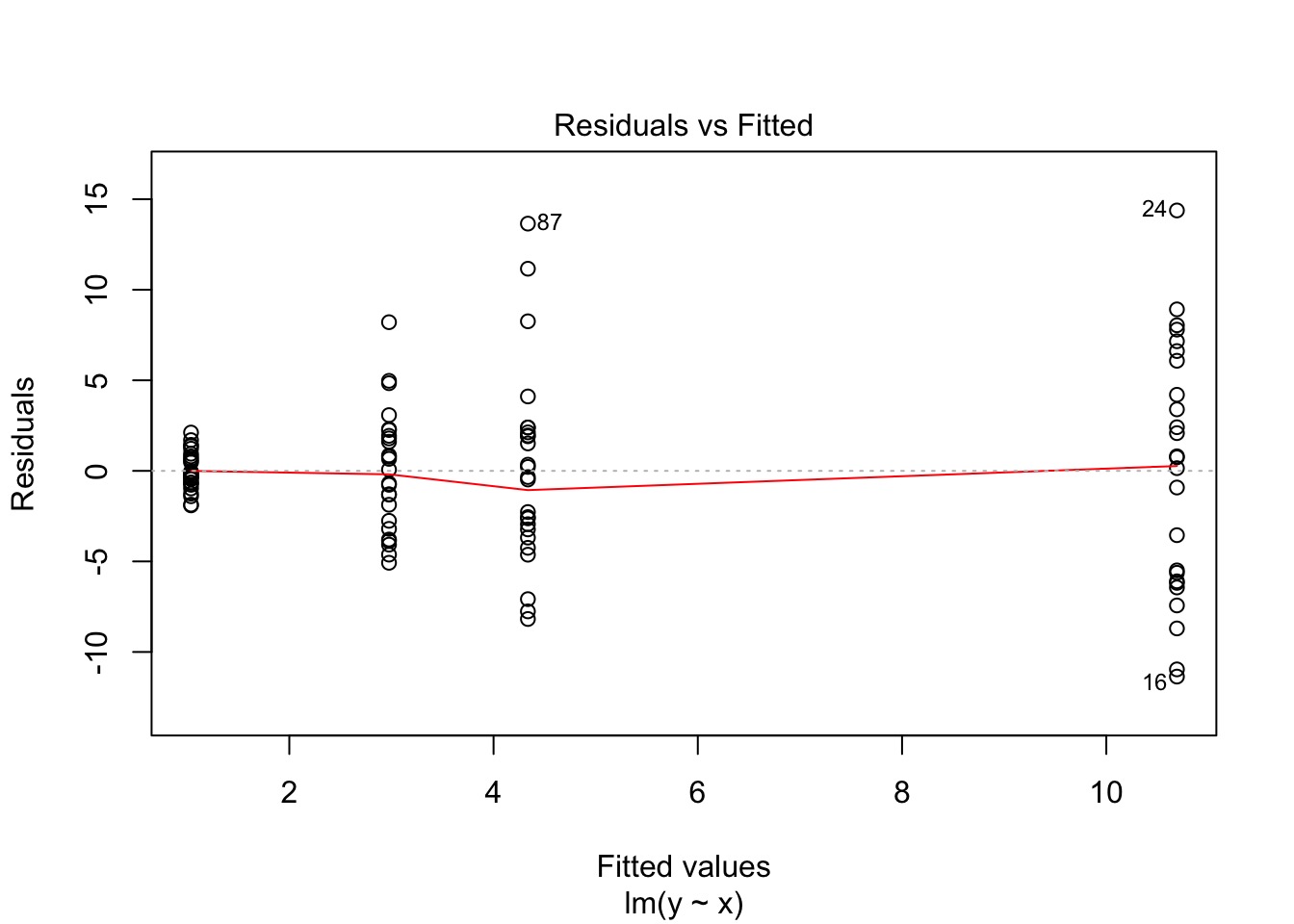
What do we do here?
Basic Princples of Ordinary Least Squares
- Y is determined by X: p(Y \(|\) X=x)
- The relationship between X and Y is Linear
- The residuals of \(\widehat{Y_i} = \beta_0 + \beta_1 X_i + \epsilon\) are normally distributed with constant variance
(i.e., \(\epsilon_i \sim\) N(0,\(\sigma\)))
Basic Principles of Ordinary Least Squares
\(\widehat{Y} = \beta_0 + \beta_1 X + \epsilon\) where \(\beta_0\) = intercept, \(\beta_1\) = slope
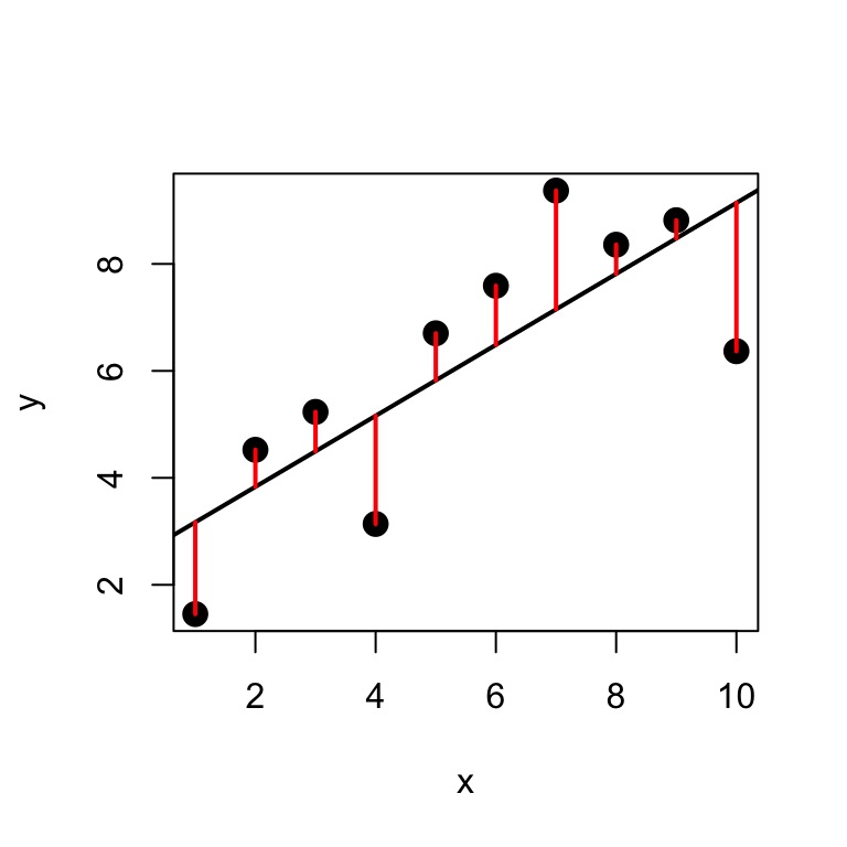
Minimize Residuals defined as \(SS_{residuals} = \sum(Y_{i} - \widehat{Y})^2\)
But…what about this?
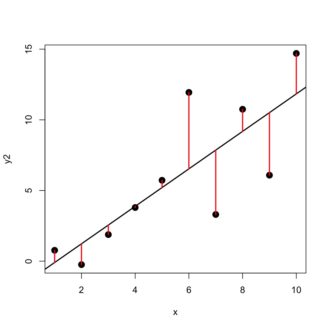
Variance-Mean Relationship
Or…what about this?
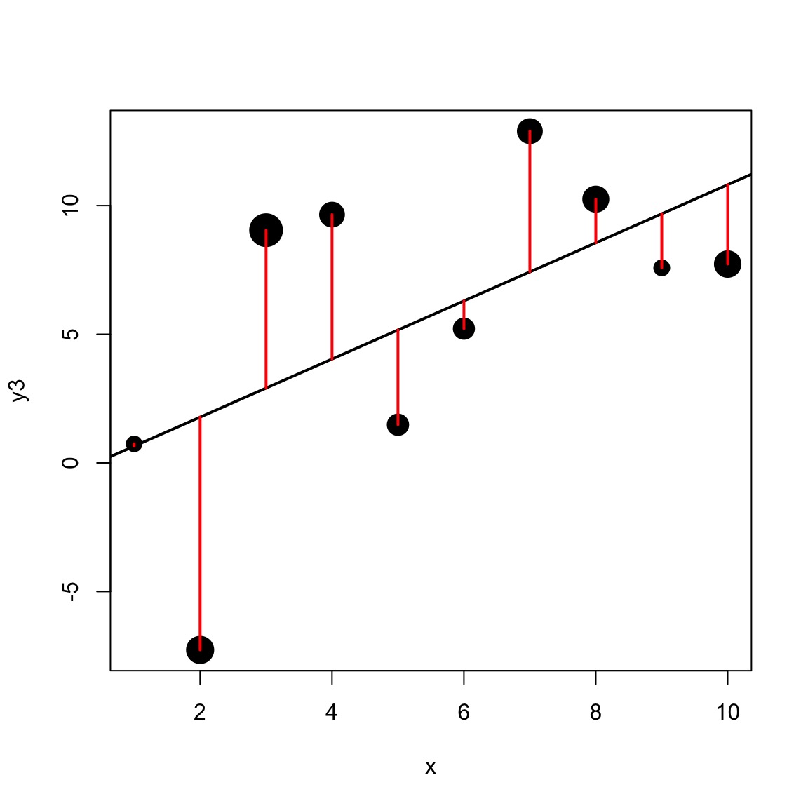
Different precision for different data points
Weighted Least Squares
Why weight?
- Minimized influence of heteroskedasticity
- Increases precision of estimates
- Decreases influence of imprecision in measurements
- Minimize sampling bias
- Other reasons to count some measurements more than others
Weighted Least Squares
\[Y_i = \beta X_i + \epsilon_i\] \[\epsilon_i \sim \mathcal{N}(0, \sigma_i)\]WLS: \(\sigma_i\) is variable
(\(I_n\) is an identity matrix with n x n dimensions)
In WLS, the diagonal of the \(\sigma\) matrix can be anything
In Generalized Least Squares, the off diagonals can be non-zero, too
How can we use weighting?
- Weighting by variance
- Mean-Variance relationship
- Unequal variance between groups
SQUID!

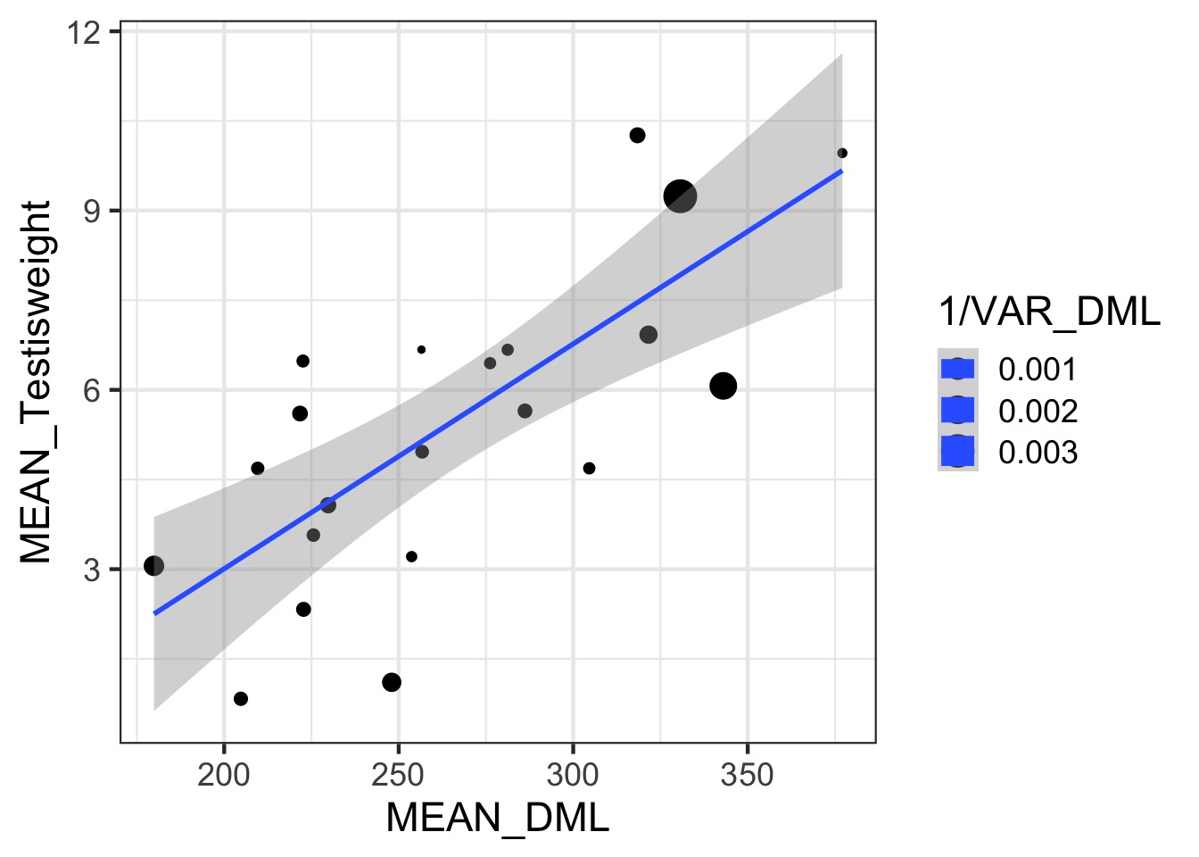
Somatic v. Reproductive Tissues: Variance
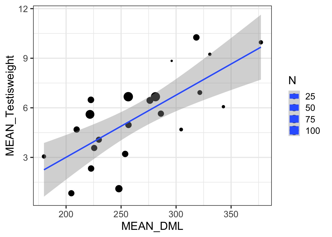
Somatic v. Reproductive Tissues: N
Weighting by Data Quality
- We typically weight by 1/variance (precision)
- Or N, or other estimate of sample precision
- This is different than variance weighted meta-analysis
- We are still estimating a residual error for fits
Implementation
Did it do anything?
No weights
| term | estimate | std.error | statistic | p.value |
|---|---|---|---|---|
| (Intercept) | -4.5177727 | 2.1081505 | -2.143003 | 0.0445948 |
| MEAN_DML | 0.0376229 | 0.0077701 | 4.842035 | 0.0000989 |
Precision Weighted
| term | estimate | std.error | statistic | p.value |
|---|---|---|---|---|
| (Intercept) | -4.518775 | 2.2041869 | -2.050087 | 0.0544130 |
| MEAN_DML | 0.037140 | 0.0074578 | 4.980010 | 0.0000831 |
Sample Size Weighted
| term | estimate | std.error | statistic | p.value |
|---|---|---|---|---|
| (Intercept) | -5.2808150 | 2.8213670 | -1.871722 | 0.0759446 |
| MEAN_DML | 0.0417104 | 0.0110373 | 3.779050 | 0.0011787 |
How can we use weighting?
- Weighting by variance
- Mean-Variance relationship
- Unequal variance between groups
Looking at Individual Squid
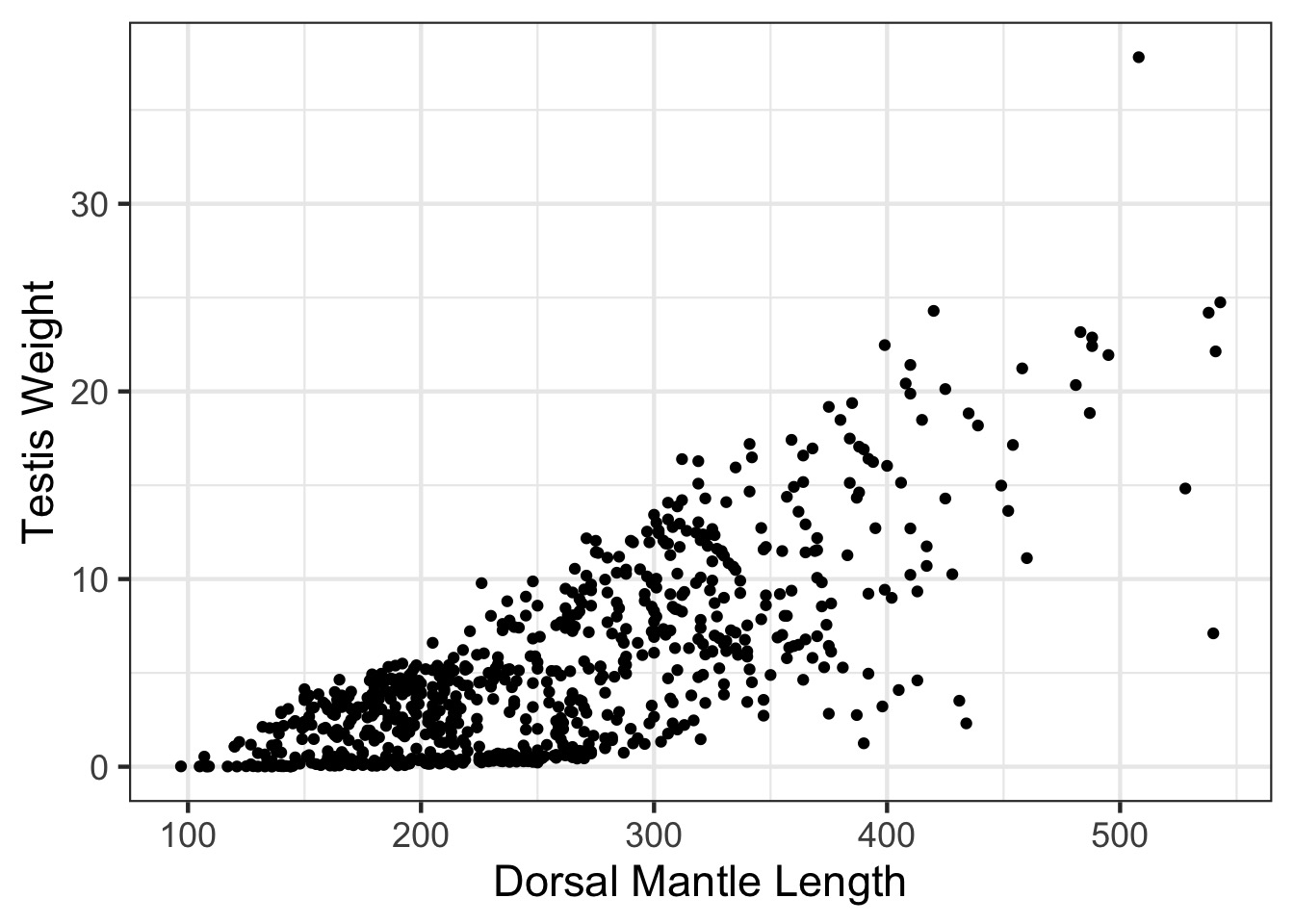
Oh, Yeah, That’s Heteroskedasticity
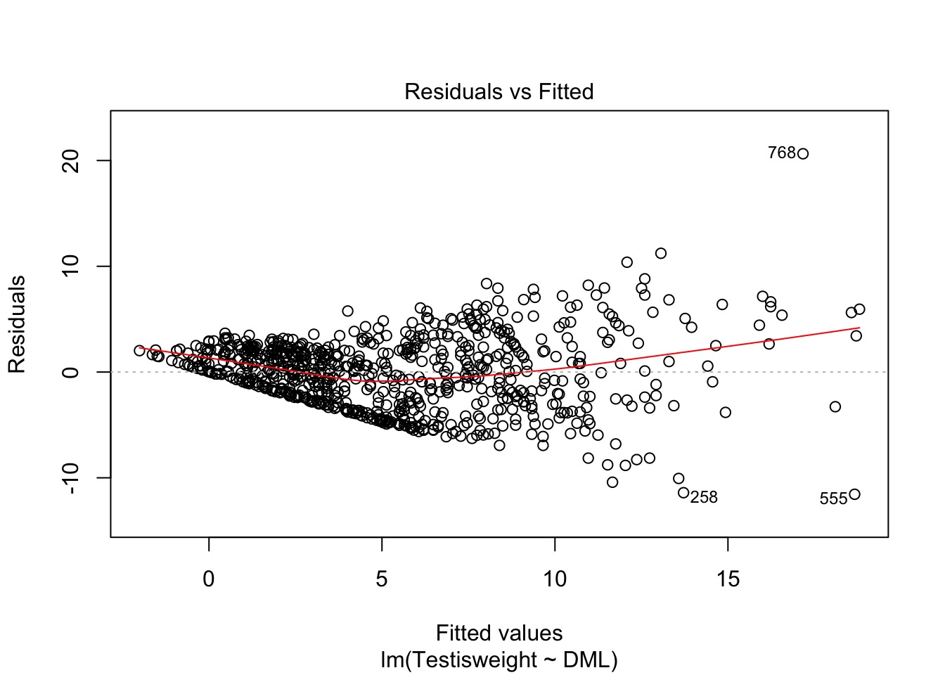
Oh, Yeah, That’s Heteroskedasticity
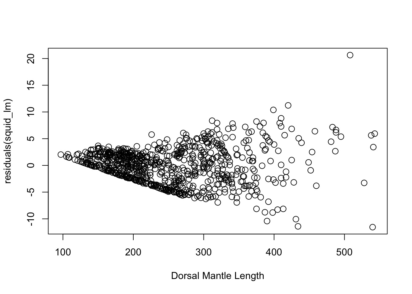
OK, But, We Need a test
- Not every case is clear-cut
- Breusch-Pagan/Godfrey/Koenker test
- Variant of White’s test (you’ll see this)
- Get squared residuals
- Regress on one or more predictors
- Results fail \(\chi^2\) test of heteroskedastic
BP Test
    studentized Breusch-Pagan test

data:  squid_lm
BP = 155.31, df = 1, p-value < 2.2e-16
Can use BP to Look at Multiple Predictors
    studentized Breusch-Pagan test

data:  squid_lm2
BP = 144.22, df = 2, p-value < 2.2e-16
Can Look at Contribution of Individual Predictors
    studentized Breusch-Pagan test

data:  squid_lm2
BP = 140.74, df = 1, p-value < 2.2e-16
    studentized Breusch-Pagan test

data:  squid_lm2
BP = 0.086946, df = 1, p-value = 0.7681
So How do we Weight This?

Weighting by a Predictor
- Need to determine the direction variance increases
- Weight by X or 1/X
- Weight by X or 1/X
- Is it a linear or nonlinear relationship between variance and X?
- Is more than one predictor influencing variance (from BP Test/Graphs)
WLS with LM
Variance increases with DML, so weight decreases
LM is LiMiting
- Need to hand-code the weights
- Diagnostic plots will still look odd
- Cannot easily combine weights from multiple predictors
Enter NLME
- NonLinear Mixed Effects Model package
- Mixed effects?! Come to BIOL609
- BUT - also has likelihood-based methods to fit WLS and GLS
- Flexible weighting specification
WLS via GLS in NLME
Note: higher value = higher variance - opposite of lm
Compare WLS and GLS
WLS with lm
t test of coefficients:

              Estimate Std. Error t value  Pr(>|t|)
(Intercept) -5.6239370  0.3382932 -16.624 < 2.2e-16 ***
DML          0.0430654  0.0014061  30.627 < 2.2e-16 ***
---
Signif. codes:  0 '***' 0.001 '**' 0.01 '*' 0.05 '.' 0.1 ' ' 1
GLS with gls
z test of coefficients:

              Estimate Std. Error z value  Pr(>|z|)
(Intercept) -5.6239370  0.3382932 -16.624 < 2.2e-16 ***
DML          0.0430654  0.0014061  30.627 < 2.2e-16 ***
---
Signif. codes:  0 '***' 0.001 '**' 0.01 '*' 0.05 '.' 0.1 ' ' 1
Different Variance Structures
VarFixed- Linear continuous varianceVarPower- Variance increases by a powerVarExp- Variance exponentiatedVarConstPower- Variance is constant + powerVarIdent- Variance differs by groupsVarComb- Combines different variance functions
Multiple Sources of Heteroskedasticity
Let’s add month! If it was another driver…
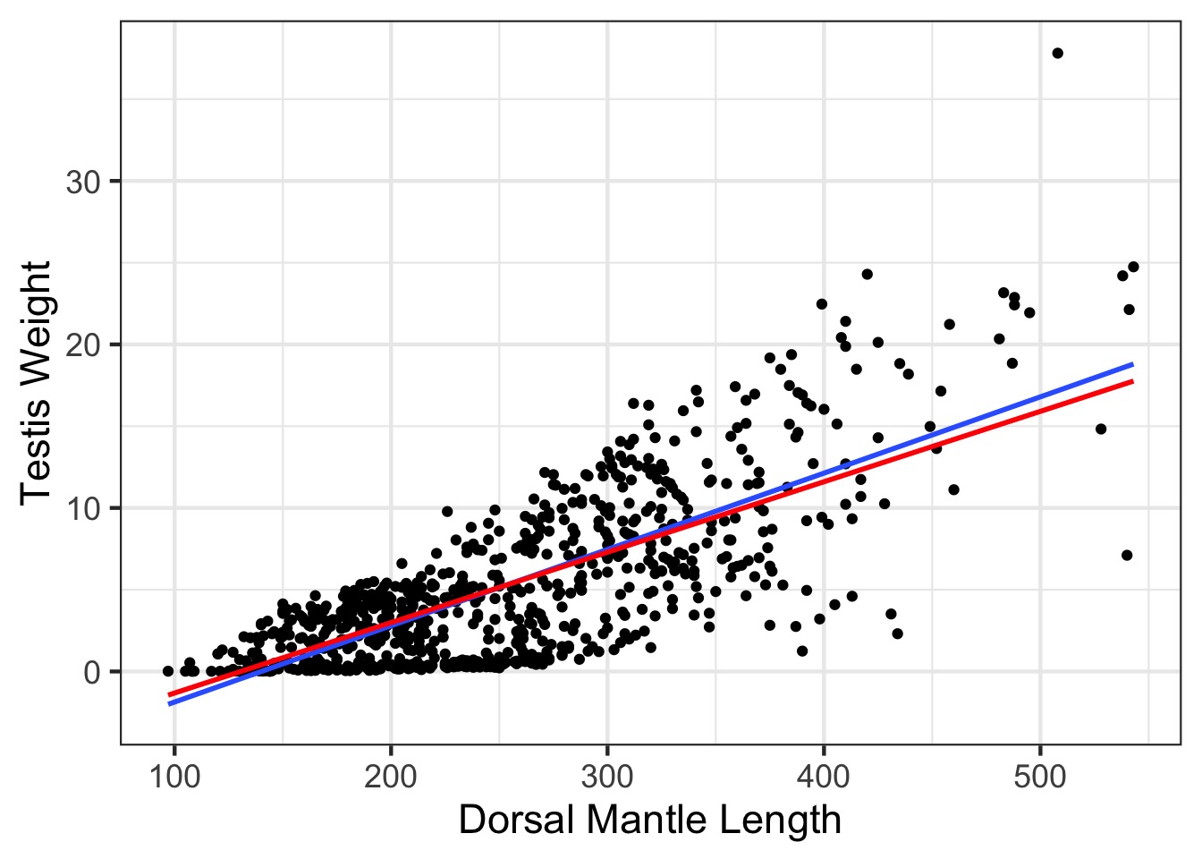
Weighted v. Naieve Fit
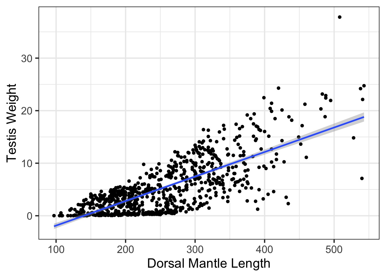
Weighted v. Naieve Fit
How can we use weighting?
- Weighting by variance
- Mean-Variance relationship
- Unequal variance between groups
Testis Weight by Month
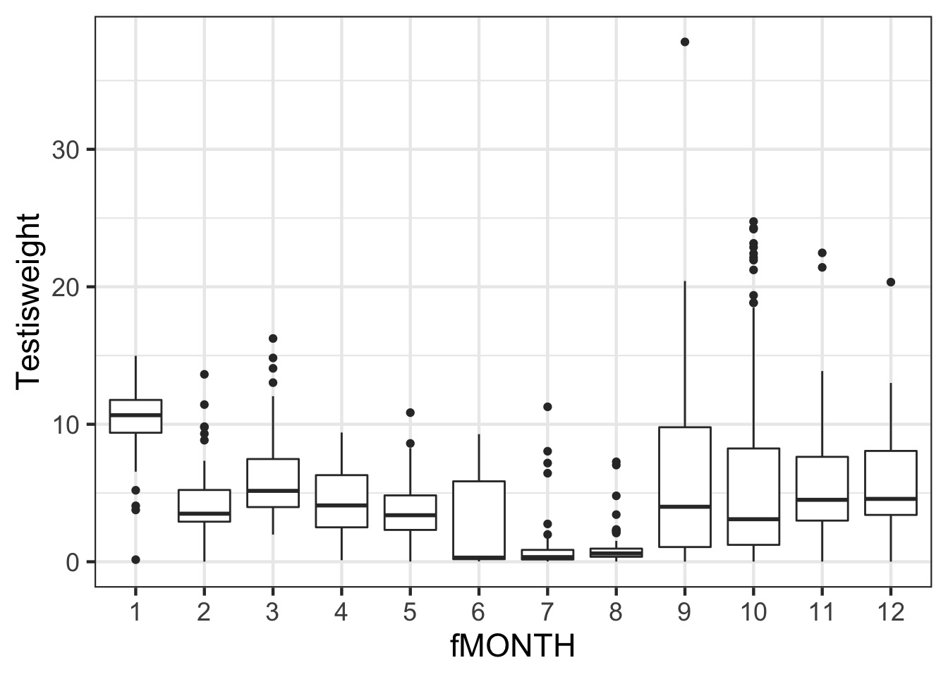
A Classic ANOVA problem
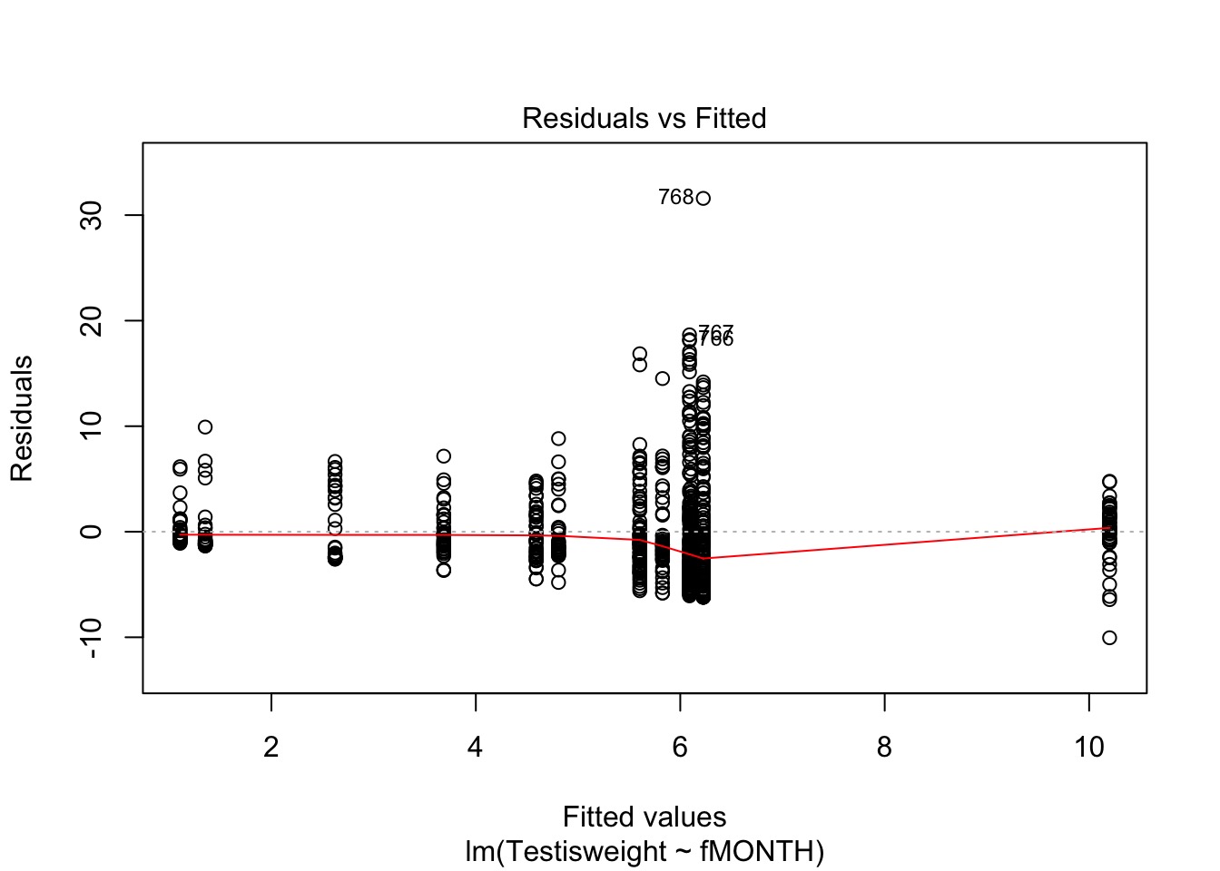
Wowsers - Unequal Variances
| MONTH | var_weight |
|---|---|
| 1 | 8.216093 |
| 2 | 9.491376 |
| 3 | 9.456260 |
| 4 | 6.663934 |
| 5 | 5.513464 |
| 6 | 10.884092 |
| 7 | 6.635753 |
| 8 | 2.274724 |
| 9 | 41.502657 |
| 10 | 46.016877 |
| 11 | 17.488115 |
| 12 | 17.734229 |
Is this a probem?
    studentized Breusch-Pagan test

data:  squid_month
BP = 68.375, df = 11, p-value = 2.485e-10
Solution: Weight by Month
- Note
1 | xform, different variance for different strata
Fit and Estimate SD
Summary of results
Generalized least squares fit by REML
  Model: Testisweight ~ fMONTH
  Data: squid
       AIC      BIC   logLik
  4307.961 4419.034 -2129.98

Variance function:
 Structure: Different standard deviations per stratum
 Formula: ~1 | fMONTH
 Parameter estimates:
        2         9        12        11         8        10         5
1.0000000 2.0910019 1.3669004 1.3573651 0.4895508 2.2018389 0.7621603
        7         6         4         1         3
0.8361283 1.0708261 0.8379142 0.9303729 0.9981331

Coefficients:
                Value Std.Error    t-value p-value
(Intercept) 10.200311 0.4272915  23.872021       0
fMONTH2     -5.391282 0.6795200  -7.933956       0
fMONTH3     -4.094684 0.5555742  -7.370184       0
fMONTH4     -5.609615 0.5722335  -9.803018       0
fMONTH5     -6.514285 0.5724283 -11.380089       0
fMONTH6     -7.577601 0.6848332 -11.064885       0
fMONTH7     -8.847744 0.6016010 -14.706997       0
fMONTH8     -9.093561 0.4757353 -19.114750       0
fMONTH9     -3.975147 0.7016302  -5.665587       0
fMONTH10    -4.109998 0.7252504  -5.667005       0
fMONTH11    -4.596277 0.6174992  -7.443373       0
fMONTH12    -4.373843 0.7482708  -5.845268       0

 Correlation:
         (Intr) fMONTH2 fMONTH3 fMONTH4 fMONTH5 fMONTH6 fMONTH7 fMONTH8
fMONTH2  -0.629
fMONTH3  -0.769  0.484
fMONTH4  -0.747  0.470   0.574
fMONTH5  -0.746  0.469   0.574   0.557
fMONTH6  -0.624  0.392   0.480   0.466   0.466
fMONTH7  -0.710  0.447   0.546   0.530   0.530   0.443
fMONTH8  -0.898  0.565   0.691   0.671   0.670   0.560   0.638
fMONTH9  -0.609  0.383   0.468   0.455   0.455   0.380   0.433   0.547
fMONTH10 -0.589  0.370   0.453   0.440   0.440   0.368   0.418   0.529
fMONTH11 -0.692  0.435   0.532   0.517   0.517   0.432   0.491   0.622
fMONTH12 -0.571  0.359   0.439   0.426   0.426   0.356   0.406   0.513
         fMONTH9 fMONTH10 fMONTH11
fMONTH2
fMONTH3
fMONTH4
fMONTH5
fMONTH6
fMONTH7
fMONTH8
fMONTH9
fMONTH10  0.359
fMONTH11  0.421   0.408
fMONTH12  0.348   0.336    0.395

Standardized residuals:
       Min         Q1        Med         Q3        Max
-3.5056018 -0.6728255 -0.3252821  0.4762647  4.9030298

Residual standard error: 3.08087
Degrees of freedom: 768 total; 756 residual
Compare with Unweighted Fit
                Model df      AIC      BIC    logLik   Test L.Ratio
squid_lm            1 13 4555.853 4616.017 -2264.926
squid_month_gls     2 24 4307.961 4419.034 -2129.980 1 vs 2 269.892
                p-value
squid_lm
squid_month_gls  <.0001
A Clammy Example: Remember your workflow!
- Clams.txt has data on the length-AFDM relationship of Wedge clames in Argentina each month.
- Useread_delimto read it in
- Evaluate the length-biomass relationship
- Test for Heteroskedasticity
- Correct for it
- Do the same for just month
- You’ll have to make it a factor
- Combine them into one model!
- usevarComb