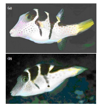
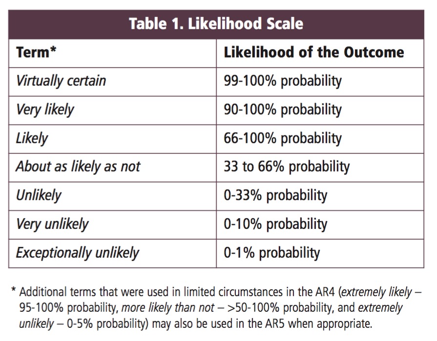
Bayesian Inference with Linear Models

class: center, middle

# Bayesian Inference with Linear Models

![:scale 55%](images/15/bayes_in_the_head.jpg)

---
class: center, middle

# Etherpad
<br><br>
.center[
### https://etherpad.wikimedia.org/p/607-bayes-lm-2020
]

---
# Puffers!

.pull-left[
- Pufferfish are toxic/harmful to predators  
<br>
- Batesian mimics gain protection from predation - why?
<br><br>
- Evolved response to appearance?
<br><br>
- Researchers tested with mimics varying in toxic pufferfish resemblance
]

.pull-right[
![:scale 80%](./images/11/puffer_mimics.jpg)
]

---
# This is our fit relationship
<img src="bayesian_lm_inference_files/figure-html/puffershow-1.png" style="display: block; margin: auto;" />

---
# Implementing the Puffer Model in brms
<br><br>

```r
puffer_brms <- brm(predators ~ resemblance, 
                   family = gaussian(link = "identity"),
                   data = puffer)
```

---
# We converge

---
# Our distribution of simulations matches observations

---
# This is what we have.... so, what can we say?

<img src="bayesian_lm_inference_files/figure-html/mcmc_params-1.png" style="display: block; margin: auto;" />
---
# Inference with a Fit Bayesian Linear Model

1. Well, what do the coefficients say?

2. What are the implications of the coefficients?

3. How well does our model fit?

4. How predictive is our model?
     - Even relative to others

---
# The Information About our Fit at 80% CI
<table>
 <thead>
  <tr>
   <th style="text-align:left;">   </th>
   <th style="text-align:right;"> Estimate </th>
   <th style="text-align:right;"> Est.Error </th>
   <th style="text-align:right;"> l-80% CI </th>
   <th style="text-align:right;"> u-80% CI </th>
   <th style="text-align:right;"> Rhat </th>
  </tr>
 </thead>
<tbody>
  <tr>
   <td style="text-align:left;"> Intercept </td>
   <td style="text-align:right;"> 1.96 </td>
   <td style="text-align:right;"> 1.65 </td>
   <td style="text-align:right;"> -0.11 </td>
   <td style="text-align:right;"> 4.05 </td>
   <td style="text-align:right;"> 1 </td>
  </tr>
  <tr>
   <td style="text-align:left;"> resemblance </td>
   <td style="text-align:right;"> 2.98 </td>
   <td style="text-align:right;"> 0.63 </td>
   <td style="text-align:right;"> 2.21 </td>
   <td style="text-align:right;"> 3.77 </td>
   <td style="text-align:right;"> 1 </td>
  </tr>
</tbody>
</table>

Note Rhat values - must = 1!!!

---

# You can think just about the Credible Intervals

.center[.middle[

|              |    10%|    90%|
|:-------------|------:|------:|
|b_Intercept   |  -0.11|   4.05|
|b_resemblance |   2.21|   3.77|
|sigma         |   2.58|   4.00|
|lp__          | -56.87| -53.92|
]]

---

# A Visual Understanding of your Coefs Can Be Helpful

---
# Inference with a Fit Bayesian Linear Model

1. Well, what do the coefficients say?

2. .red[What are the implications of the coefficients?]

3. How well does our model fit?

4. How predictive is our model?
     - Even relative to others
---

# How do you use your posterior?

1. What is the weight of the tail on the other side of 0?
     - Hey....is that.... cheating?
     - Maybe, but...
     - you can talk in terms of degree of belief in the direction of your trend

2. What is the weight of the posterior over a range of values?

3. What is the weight of a posterior &gte; a certain value?

---
# What is the weight of the tail less that 0?

Weight of Intercept &le; 0? 0.1165

Weight of Slope &le; 0? 0.00125

---

# What is the probability that the slope is between 2 and 4?

Weight of Slope between 2 and 4: 0.894

---

# Talking about Uncertainty the IPCC Way

.center[
![:scale 80%](images/15/ipcc_uncertainty_ar5.jpg)
]

---

# Visualize the mean fit...
<img src="bayesian_lm_inference_files/figure-html/fit_fig-1.png" style="display: block; margin: auto;" />

---

# And the distributions of fits
<img src="bayesian_lm_inference_files/figure-html/dist_fit-1.png" style="display: block; margin: auto;" />

---
# And the distributions of fits
<img src="bayesian_lm_inference_files/figure-html/unnamed-chunk-1-1.png" style="display: block; margin: auto;" />

---

# Add the distribution of predictions
<img src="bayesian_lm_inference_files/figure-html/puffer_pred_brms-1.png" style="display: block; margin: auto;" />

---

# What does visualization do for you?

1. Shows trends

2. Shows variability in precision or in prediction

3. Shows you where you can frame your degree of belief

---
# Inference with a Fit Bayesian Linear Model

1. Well, what do the coefficients say?

2. What are the implications of the coefficients?

3. .red[How well does our model fit?]

4. How predictive is our model?
     - Even relative to others
     
---

# Bayesian `$R^2$`

Classically, we use

`$$1 - \frac{\sigma^2}{s^2_{data}}$$`

$$ = \frac{variance \, explained}{total \, variance}$$
But....

- `$R^2$` under some draws can be negative 
     - Consider a draw where the slope is *VERY* steep relative to a flat relationship
     - Consider a very very strong prior
     
- `$R^2$` depends on the data, and thus isn't a good absolute measure of model goodness of fit

---

# Bayesian `$R^2$`

`$$\large R^2_{bayes} = \frac{variance \, explained}{variance \, explained + residual \, variance}$$`

- Cannot be negative

- Based on model fit and draws from posterior relative to data

---

# Bayesian `$R^2$` Visualized

<table>
 <thead>
  <tr>
   <th style="text-align:left;">   </th>
   <th style="text-align:right;"> Estimate </th>
   <th style="text-align:right;"> Est.Error </th>
   <th style="text-align:right;"> Q10 </th>
   <th style="text-align:right;"> Q90 </th>
  </tr>
 </thead>
<tbody>
  <tr>
   <td style="text-align:left;"> R2 </td>
   <td style="text-align:right;"> 0.574884 </td>
   <td style="text-align:right;"> 0.1104888 </td>
   <td style="text-align:right;"> 0.4292734 </td>
   <td style="text-align:right;"> 0.6868686 </td>
  </tr>
</tbody>
</table>

---
# Inference with a Fit Bayesian Linear Model

1. Well, what do the coefficients say?

2. What are the implications of the coefficients?

3. How well does our model fit?

4. .red[How predictive is our model?
  - Even relative to others
]

---

# The Return of Cross-Validation!

- We can calculate MSE of refit models.... but we need something more general

- Enter the Pointwise Predictive Density (ELPD)

---

# The Log Pointwise Predictive Density

`$$\large lppd = \sum_i log \sum_s {p(y_i | \theta_s)}$$`

- We take the log of the sum of the pointwise predictive density for all paramater values drawn from a chain

- We then sum this over *all* data points

- Kinda nice, no?

- It will have the same problem as MSE, etc., for overfitting
     - More parameters = better fit = higher lppd!
     
---

# Solutions to Overfitting

- An AIC-like score

- LOO Cross Validation

- K-fold Cross validation

---
# Penalty for Too Many Parameters

- As # of parameters goes up, lppd goes up

- BUT - as # of parameters goes up, variance in lppd for each point goes up
     - More parameters, higher SE per parameter, more variance in lppd

`$$\large penalty = \sum_ivar(lppd_i)$$`
--

- akin to # of parameters penalty

---
# The Widely Applicable Information Criterion

`$$\LARGE WAIC = -2(lppd - penalty)$$`

- Akin to AIC

- Can be calculated point by point

- But.... sensitive to extreme lppds

---
# WAIC from our Puffers

```r
waic(puffer_brms)
```

```
Warning: 
1 (5.0%) p_waic estimates greater than 0.4. We recommend trying loo instead.
```

```

Computed from 4000 by 20 log-likelihood matrix

Estimate  SE
elpd_waic    -52.7 2.7
p_waic         2.5 0.7
waic         105.5 5.3

1 (5.0%) p_waic estimates greater than 0.4. We recommend trying loo instead. 
```

---
# WAIC Problems from our Puffers
<img src="bayesian_lm_inference_files/figure-html/waicplot-1.png" style="display: block; margin: auto;" />

---
# WAIC Problems from our Puffers
<img src="bayesian_lm_inference_files/figure-html/waicplot_2-1.png" style="display: block; margin: auto;" />

---

# LOO Cross-validation!

- OMG! We have to refit out model for every point? Didn't one take enough?

- Fear not, there is a solution!

- The posterior, p(H|D), is the *product* of the posterior for all data points

`$$p(\theta|y) = \prod p(\theta|y_i)$$`
--

- So, We can get our PPD for leaving out one data point by dividing the posterior by `$p(\theta | y_i)$` - so deliciously simple!

- But, what if the importance of a given point is anomolusly large?

- Introducing, pareto smoothing

---

# The Pareto Distribution for Importance

- Vilfredo Pareto introduced the Pareto distribution to describe the distribution of wealth in a society
     - Leads to 80:20 rule, 80% of outcomes due to 20% of causes

- More commonly, a curve to describe relative importance

- We use it to smooth the relative importance values of each `$lpd_i$`

---

# The Pareto Distribution for Importance

---

# LOO!

```r
loo(puffer_brms)
```

```

Computed from 4000 by 20 log-likelihood matrix

Estimate  SE
elpd_loo    -52.8 2.7
p_loo         2.6 0.7
looic       105.6 5.4
------
Monte Carlo SE of elpd_loo is 0.0.

All Pareto k estimates are good (k < 0.5).
See help('pareto-k-diagnostic') for details.
```

- k is an estimate of our shape parameter for the Pareto distribution

- if k > 0.5, we use K-Fold Cross validationt

---

# K-fold CV!

```r
kfold(puffer_brms, K = 5)
```

```

Based on 5-fold cross-validation

Estimate  SE
elpd_kfold    -52.8 2.6
p_kfold          NA  NA
kfoldic       105.5 5.2
```

Expensive, though, as you actually have to refit for each fold

---

# Can then use LOO, WAIC, etc. to compare models

```r
puffer_cubic <- brm(predators ~ poly(resemblance, 3),
                     family = gaussian(link = "identity"),
                     data = puffer)
```

```r
puffer_loo <- loo(puffer_brms)
puffer_cubic_loo <- loo(puffer_cubic)

loo_compare(puffer_loo, puffer_cubic_loo)
```

```
             elpd_diff se_diff
puffer_brms   0.0       0.0   
puffer_cubic -1.4       1.3   
```
---

# Wrapping up...

- We can use many of the same inferential frameworks as before, but...

- The difference is that now we can begin to talk about our inferences in degree of certainty

- To adopt a Bayesian viewpoint on the world is to abandon the idea of a "True" parameter value

- We now see parameters as having a distribution

- The null is no longer of interest, but rather the probability of possibility is what drives us