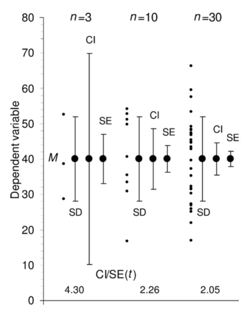
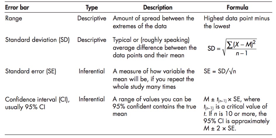
Sampling Estimate, Precision, and Simulation

# Sampling Estimates, Precision, and Simulation

![](images/04/target.png)

### Biol 607
---

# Today's Etherpad
 .center[.large[https://etherpad.wikimedia.org/p/sampling-2020]]

---

# Estimation and Precision

2. Simulation, Precision, and Sample Size Estimation

3. Bootstrapping our Way to Confidence

]
---
# Last Time: Sample Versus Population

---

# Sample Properties: **Mean**

`$$\bar{x} = \frac{ \displaystyle \sum_{i=1}^{n}{x_{i}} }{n}$$`

`$\large \bar{x}$` - The average value of a sample  
`$x_{i}$` - The value of a measurement for a single individual   
n - The number of individuals in a sample  
&nbsp;  
`$\mu$` - The average value of a population  
(Greek = population, Latin = Sample)

---
class: center, middle

# Our goal is to get samples representative of a population, and estimate population parameters. We assume a **distribution** of values to the population.

---
# Probability Distributions
<img src="04_simulation_estimation_x_files/figure-html/normplot-1.png" style="display: block; margin: auto;" />

---

# Probability Distributions Come in Many Shapes

---

# The Normal (Gaussian) Distribution

- Arises from some deterministic value and many small additive deviations
- VERY common
---
class: center

# Understanding Gaussian Distributions with a Galton Board (Quinqunx)

---

# We see this pattern everywhere - the Random or Drunkard's Walk

```r
one_path <- function(steps){
 
 each_step <- c(0, runif(steps, min = -1, max = 1))

path <- cumsum(each_step)
 
 return(path)
}
```

1. Input some number of steps to take

2. Make a vector of 0 and a bunch of random numbers from -1 to 1

3. Take the cummulative sum across the vector to represent the path

4. Return the path vector

---

# 1000 Simulated Random Walks to Normal Homes
<img src="04_simulation_estimation_x_files/figure-html/all_walks-1.png" style="display: block; margin: auto;" />

---

# A Normal Result for Final Position

---

# Normal distributions
<img src="04_simulation_estimation_x_files/figure-html/normplot-1.png" style="display: block; margin: auto;" />

- Results from additive accumulation of many small errors
- Defined by a mean and standard deviation: `$N(\mu, \sigma)$`
- 2/3 of data is within 1 SD of the mean
- Values are peaked without **skew** (skewness = 0)
- Tails are neither too thin nor too fat (**kurtosis** = 0)
---

# Estimation and Precision

2. .red[Simulation, Precision, and Sample Size Estimation]

3. Bootstrapping our Way to Confidence

]

---
class: middle, center

# The Eternal Question: What should my sample size be?

---

# Let's find out
.large[
1. Get in groups of 3 
2. Ask each other your age. Report the mean to me. 
3. Now get into another group of five, and do the same. 
4. Now get into another group of ten, and do the same. 
]
---

# We simulated sampling from our class population!

---
# What if We Could Pretend to Sample?
.large[
- Assume the distribution of a population

- Draw simulated 'samples' from the population at different sample sizes

- Examine when an estimated property levels off or precision is sufficient
      - Here we define Precision as 1/variance at a sample size
]
---
background-image: url(images/04/is-this-a-simulation.jpg)
background-position: center
background-size: cover

---

background-image: url(images/04/firefly-ship.jpg)
background-position: center
background-size: cover
class: center

# .inverse[Let's talk Firefly]

---
background-image: url(images/04/fireflies-1500x1000.jpg)
background-position: center
background-size: cover

---
# Start With a Population...

Mean of Firefly flashing times: 95.9428571  
SD of Firefly flasing times: 10.9944982

So assuming a normal distribution...

---
# Choose a Random Sample - n=5?

Mean of Firefly flashing times: 95.9428571  
SD of Firefly flasing times: 10.9944982  
So assuming a normal distribution...

```r
rnorm(n = 5,
      mean = mean(firefly$flash.ms),
      sd = sd(firefly$flash.ms)
```
---

# Calculate Sample Mean

Mean of Firefly flashing times: 95.9428571  
SD of Firefly flasing times: 10.9944982  
So assuming a normal distribution...

--
Rinse and repeat...

---
# How Good is our Sample Size for Estimating a Mean?

---
# Where does the variability level off?
<img src="04_simulation_estimation_x_files/figure-html/dist_sim_stop-1.png" style="display: block; margin: auto;" />

---
# Many Ways to Visualize

---
# Where does the variability level off?

```
# A tibble: 99 x 2
 sampSize mean_sim_sd
 <int> <dbl>
 1 96 1.10
 2 100 1.11
 3 92 1.12
 4 95 1.12
 5 97 1.13
 6 89 1.13
 7 93 1.13
 8 98 1.13
 9 99 1.14
10 91 1.17
# … with 89 more rows
```

---

# Visualize Variability in Estimate of Mean

--
.large[What is acceptable to you? And/or relative to the Mean?]

---
class: center, middle
# **Central Limit Theorem** The distribution of means of a sufficiently large sample size will be approximately normal

https://istats.shinyapps.io/sampdist_cont/

---
class: center, middle
# The Standard Error
 
.large[
A standard error is the standard deviation of an estimated parameter if we were able to sample it repeatedly. 
]

---

# But, I only Have One Sample? How can I know my SE for my mean or any other parameter?

---

# Estimation and Precision

2. Simulation, Precision, and Sample Size Estimation

3. .red[Bootstrapping our Way to Confidence]

]
---

# The Bootstrap
.large[

- We can resample our sample some number of times with replacement

- This resampling with replacement is called **bootstrapping**

- One replicate simulation is one **bootstrap**
]

---
# One Bootstrap Sample in R

```r
# One bootstrap
sample(firefly$flash.ms, size = nrow(firefly), replace = TRUE)
```

```
 [1]  95  95  85  87  86  95  80 109  86  95 106  96 109  88  86  87 112  92  79
[20] 116  89  92  98 112 113 118  94  94  95  86  87  94 118 109  98
```

---

# Boostrapped Estimate of a SE
- We can calculate the Standard Deviation of a sample statistic from replicate bootstraped samples

- This is called the botstrapped **Standard Error** of the estimate

```r
one_boot <- function(){
 sample(firefly$flash.ms, size = nrow(firefly), replace = TRUE)
}

boot_means <- replicate(1000, mean(one_boot()))

sd(boot_means)
```

```
[1] 1.816216
```

---
class: large

# So I always have to boostrap Standard Errors?

## .center[**No**]

Many common estimates have formulae, e.g.:

`$$SE_{mean} = \frac{s}{\sqrt(n)}$$`

Boot SEM: Boot SEM: 1.816, Est. SEM: 2

---

# Bootstrapping to Estimate Precision of a Non-Standard Metric

SE of the SD = 1.101

---
class: large

# Standard Error as a Measure of Confidence
--

- We have drawn our SE from a **sample** - not the **population**

- Our estimate ± 1 SE tells us 2/3 of the **estimates** we could get by resampling this sample

- This is **not** 2/3 of the possible **true parameter values**

- Rather, if we were to sample the population many many times, 2/3 of the time, this interval will contain the true value

---

# Confidence Intervals

- ~2 SE = 95% Confidence Interval

- Best to view these as a measure of precision of your estimate

- And remember, if you were able to do the sampling again and again and again, some fraction of your intervals would contain a true value
]
---

# Let's see this in action

### .center[.middle[https://istats.shinyapps.io/ExploreCoverage/]]

---

# Frequentist Philosophy

.large[The ideal of drawing conclusions from data based on properties derived from theoretical resampling is fundamentally **frequentist** - i.e., assumes that we can derive truth by observing a result with some frequency in the long run.]

---
# A Final Note: SE, SD, CIs....
![:scale 55%](images/04/cumming_comparison_2007.jpg)
.bottom[.small[.left[[Cumming et al. 2007 Figure 4](http://byrneslab.net/classes/biol-607/readings/Cumming_2007_error.pdf)]]]
---
# SE, SD, CIs....
![:scale 75%](images/04/cumming_table_2007.jpg)

.bottom[.small[.left[[Cumming et al. 2007 Table 1](http://byrneslab.net/classes/biol-607/readings/Cumming_2007_error.pdf)]]]