After the ANOVA

Outline

https://etherpad.wikimedia.org/p/607-anova

Beyond ANOVA: T and Posthoc Tests
ANOVA in a Likelihood and Bayesian Context

Categorical Predictors: Gene Expression and Mental Disorders

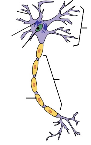
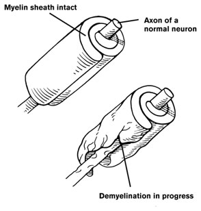
The data

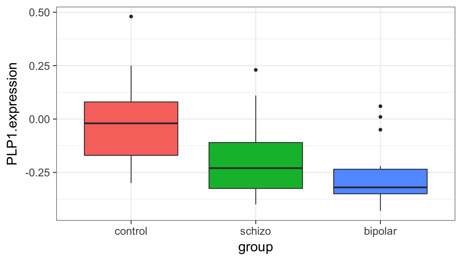
Comparison of Means

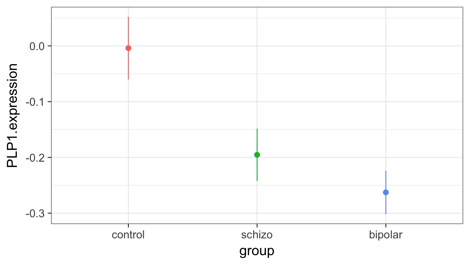
Means Model

\[\large y_{ij} = \mu + \alpha_{i} + \epsilon_{ij}, \qquad \epsilon_{ij} \sim N(0, \sigma^{2} )\]

Different mean for each group

Focus is on specificity of a categorical predictor

Questions we could ask

Does your model explain variation in the data?
Are your coefficients different from 0?
How much variation is retained by the model?
How confident can you be in model predictions?

Testing the Model

Ho = The model predicts no variation in the data.

Ha = The model predicts variation in the data.

F-Tests

F = Mean Square Variability Explained by Model / Mean Square Error

DF for Numerator = k-1 DF for Denominator = n-k
k = number of groups, n = sample size

Questions we could ask

Does your model explain variation in the data?
Are your coefficients different from 0?
How much variation is retained by the model?
How confident can you be in model predictions?
Are groups different from each other

Questions we could ask

Does your model explain variation in the data?
Are your coefficients different from 0?
How much variation is retained by the model?
How confident can you be in model predictions?
Are groups different from each other

ANOVA

	Df	Sum Sq	Mean Sq	F value	Pr(>F)
group	2	0.5402533	0.2701267	7.823136	0.0012943
Residuals	42	1.4502267	0.0345292	NA	NA

Questions we could ask

Does your model explain variation in the data?
Are your coefficients different from 0?
How much variation is retained by the model?
How confident can you be in model predictions?
Are groups different from each other

Questions we could ask

Does your model explain variation in the data?
Are your coefficients different from 0?
How much variation is retained by the model?
How confident can you be in model predictions?
Are groups different from each other

ANOVA, F, and T-Tests

F-Tests	T-Tests
Tests if data generating process different than error	Tests if parameter is different from 0

Essentially comparing a variation explained by a model with versus without a data generating process included.

The Coefficients

	Estimate	Std. Error	t value	Pr(>\|t\|)
(Intercept)	-0.0040000	0.0479786	-0.0833705	0.9339531
groupschizo	-0.1913333	0.0678520	-2.8198628	0.0073015
groupbipolar	-0.2586667	0.0678520	-3.8122186	0.0004442

Treatment contrasts - set one group as a baseline
Useful with a control

Default “Treatment” Contrasts

        schizo bipolar
control      0       0
schizo       1       0
bipolar      0       1

Actual Group Means Compared to 0

	Estimate	Std. Error	t value	Pr(>\|t\|)
groupcontrol	-0.0040000	0.0479786	-0.0833705	0.9339531
groupschizo	-0.1953333	0.0479786	-4.0712586	0.0002022
groupbipolar	-0.2626667	0.0479786	-5.4746618	0.0000023

But which groups are different from each other?

Many T-tests….mutiple comparisons!

The Problem of Multiple Comparisons

Solutions to Multiple Comparisons and Family-wise Error Rate?

Ignore it - a test is a test
- a priori contrasts
- Least Squares Difference test

Lower your \(\alpha\) given m = # of comparisons
- Bonferroni \(\alpha/m\)
- False Discovery Rate \(k\alpha/m\) where k is rank of test

Other multiple comparinson correction
- Tukey’s Honestly Significant Difference

ANOVA is an Omnibus Test

Remember your Null:
\[H_{0} = \mu_{1} = \mu{2} = \mu{3} = ...\]

This had nothing to do with specific comparisons of means.

A priori contrasts

Specific sets of a priori null hypotheses: \[\mu_{1} = \mu{2}\]
\[\mu_{1} = \mu{3} = ...\]

Use t-tests.

A priori contrasts

lm model parameter contrast

  Contrast   S.E.  Lower Upper    t df Pr(>|t|)
1    0.191 0.0679 0.0544 0.328 2.82 42   0.0073

A priori contrasts

lm model parameter contrast

                   Contrast   S.E.  Lower Upper    t df Pr(>|t|)
Control v. Schizo     0.191 0.0679 0.0544 0.328 2.82 42   0.0073
Control v. Bipolar    0.259 0.0679 0.1217 0.396 3.81 42   0.0004

Note: can only do k-1, as each takes 1df

Orthogonal A priori contrasts

Sometimes you want to test very specific hypotheses about the structure of your groups

                     control schizo bipolar
Control v. Disorders       1   -0.5    -0.5
Bipolar v. Schizo          0    1.0    -1.0

Note: can only do k-1, as each takes 1df

Orthogonal A priori contrasts with Grouping


     Simultaneous Tests for General Linear Hypotheses

Fit: lm(formula = PLP1.expression ~ group, data = brainGene)

Linear Hypotheses:
                          Estimate Std. Error t value Pr(>|t|)  
Control v. Disorders == 0   0.2210     0.1018    2.17     0.07 .
Bipolar v. Schizo == 0      0.0673     0.0679    0.99     0.54  
---
Signif. codes:  0 '***' 0.001 '**' 0.01 '*' 0.05 '.' 0.1 ' ' 1
(Adjusted p values reported -- single-step method)

Post hoc contrasts

I want to test all possible comparisons!

No Correction: Least Square Differences

pairwise.t.test(brainGene$PLP1.expression, brainGene$group, 
                p.adjust.method="none")


    Pairwise comparisons using t tests with pooled SD 

data:  brainGene$PLP1.expression and brainGene$group 

        control schizo
schizo  0.007   -     
bipolar 4e-04   0.327 

P value adjustment method: none

P-Value Adjustments

Bonferroni : \(\alpha_{adj} = \frac{\alpha}{m}\) where m = # of tests
- VERY conservative

False Discovery Rate: \(\alpha_{adj} = \frac{k\alpha}{m}\)
- Order your p values from smallest to largest, rank = k,
- Adjusts for small v. large p values
- Less conservative

Other Methods: Sidak, Dunn, Holm, etc.
We’re very focused on p here!

Bonferroni Corrections

pairwise.t.test(brainGene$PLP1.expression, brainGene$group, 
                p.adjust.method="bonferroni")


    Pairwise comparisons using t tests with pooled SD 

data:  brainGene$PLP1.expression and brainGene$group 

        control schizo
schizo  0.022   -     
bipolar 0.001   0.980 

P value adjustment method: bonferroni

FDR

pairwise.t.test(brainGene$PLP1.expression, brainGene$group, 
                p.adjust.method="fdr")


    Pairwise comparisons using t tests with pooled SD 

data:  brainGene$PLP1.expression and brainGene$group 

        control schizo
schizo  0.011   -     
bipolar 0.001   0.327 

P value adjustment method: fdr

Other Methods Use Critical Values

Tukey’s Honestly Significant Difference
Dunnet’s Test for Comparison to Controls
Ryan’s Q (sliding range)
etc…

Tukey’s Honestly Significant Difference

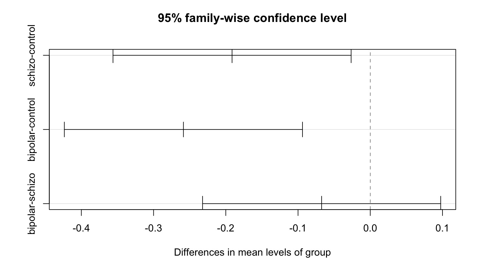
  Tukey multiple comparisons of means
    95% family-wise confidence level

Fit: aov(formula = PLP1.expression ~ group, data = brainGene)

$group
                   diff    lwr     upr p adj
schizo-control  -0.1913 -0.356 -0.0265 0.020
bipolar-control -0.2587 -0.424 -0.0938 0.001
bipolar-schizo  -0.0673 -0.232  0.0975 0.586

Visualizing Comparisons

Final Notes of Caution

Often you DO have a priori contrasts in mind
If you reject Ho with ANOVA, differences between groups exist
Consider Type I v. Type II error before correcting

Outline

https://etherpad.wikimedia.org/p/607-anova

Beyond ANOVA: T and Posthoc Tests
ANOVA in a Likelihood and Bayesian Context

Fitting an ANOVA model with Likelihood

brain_lik <- glm(PLP1.expression ~ group,
                 family=gaussian(),
                 data = brainGene)

\(\chi^2\) LR Test and ANOVA

	LR Chisq	Df	Pr(>Chisq)
group	15.6	2	4e-04

Likelihood and Posthocs


     Simultaneous Tests for General Linear Hypotheses

Multiple Comparisons of Means: Tukey Contrasts


Fit: lm(formula = PLP1.expression ~ group, data = brainGene)

Linear Hypotheses:
                       Estimate Std. Error t value Pr(>|t|)   
schizo - control == 0   -0.1913     0.0679   -2.82   0.0196 * 
bipolar - control == 0  -0.2587     0.0679   -3.81   0.0012 **
bipolar - schizo == 0   -0.0673     0.0679   -0.99   0.5857   
---
Signif. codes:  0 '***' 0.001 '**' 0.01 '*' 0.05 '.' 0.1 ' ' 1
(Adjusted p values reported -- single-step method)

BANOVA


SAMPLING FOR MODEL 'continuous' NOW (CHAIN 1).

Chain 1, Iteration:    1 / 2000 [  0%]  (Warmup)
Chain 1, Iteration:  200 / 2000 [ 10%]  (Warmup)
Chain 1, Iteration:  400 / 2000 [ 20%]  (Warmup)
Chain 1, Iteration:  600 / 2000 [ 30%]  (Warmup)
Chain 1, Iteration:  800 / 2000 [ 40%]  (Warmup)
Chain 1, Iteration: 1000 / 2000 [ 50%]  (Warmup)
Chain 1, Iteration: 1001 / 2000 [ 50%]  (Sampling)
Chain 1, Iteration: 1200 / 2000 [ 60%]  (Sampling)
Chain 1, Iteration: 1400 / 2000 [ 70%]  (Sampling)
Chain 1, Iteration: 1600 / 2000 [ 80%]  (Sampling)
Chain 1, Iteration: 1800 / 2000 [ 90%]  (Sampling)
Chain 1, Iteration: 2000 / 2000 [100%]  (Sampling)
 Elapsed Time: 0.080866 seconds (Warm-up)
               0.08541 seconds (Sampling)
               0.166276 seconds (Total)


SAMPLING FOR MODEL 'continuous' NOW (CHAIN 2).

Chain 2, Iteration:    1 / 2000 [  0%]  (Warmup)
Chain 2, Iteration:  200 / 2000 [ 10%]  (Warmup)
Chain 2, Iteration:  400 / 2000 [ 20%]  (Warmup)
Chain 2, Iteration:  600 / 2000 [ 30%]  (Warmup)
Chain 2, Iteration:  800 / 2000 [ 40%]  (Warmup)
Chain 2, Iteration: 1000 / 2000 [ 50%]  (Warmup)
Chain 2, Iteration: 1001 / 2000 [ 50%]  (Sampling)
Chain 2, Iteration: 1200 / 2000 [ 60%]  (Sampling)
Chain 2, Iteration: 1400 / 2000 [ 70%]  (Sampling)
Chain 2, Iteration: 1600 / 2000 [ 80%]  (Sampling)
Chain 2, Iteration: 1800 / 2000 [ 90%]  (Sampling)
Chain 2, Iteration: 2000 / 2000 [100%]  (Sampling)
 Elapsed Time: 0.068858 seconds (Warm-up)
               0.063094 seconds (Sampling)
               0.131952 seconds (Total)


SAMPLING FOR MODEL 'continuous' NOW (CHAIN 3).

Chain 3, Iteration:    1 / 2000 [  0%]  (Warmup)
Chain 3, Iteration:  200 / 2000 [ 10%]  (Warmup)
Chain 3, Iteration:  400 / 2000 [ 20%]  (Warmup)
Chain 3, Iteration:  600 / 2000 [ 30%]  (Warmup)
Chain 3, Iteration:  800 / 2000 [ 40%]  (Warmup)
Chain 3, Iteration: 1000 / 2000 [ 50%]  (Warmup)
Chain 3, Iteration: 1001 / 2000 [ 50%]  (Sampling)
Chain 3, Iteration: 1200 / 2000 [ 60%]  (Sampling)
Chain 3, Iteration: 1400 / 2000 [ 70%]  (Sampling)
Chain 3, Iteration: 1600 / 2000 [ 80%]  (Sampling)
Chain 3, Iteration: 1800 / 2000 [ 90%]  (Sampling)
Chain 3, Iteration: 2000 / 2000 [100%]  (Sampling)
 Elapsed Time: 0.054466 seconds (Warm-up)
               0.096178 seconds (Sampling)
               0.150644 seconds (Total)


SAMPLING FOR MODEL 'continuous' NOW (CHAIN 4).

Chain 4, Iteration:    1 / 2000 [  0%]  (Warmup)
Chain 4, Iteration:  200 / 2000 [ 10%]  (Warmup)
Chain 4, Iteration:  400 / 2000 [ 20%]  (Warmup)
Chain 4, Iteration:  600 / 2000 [ 30%]  (Warmup)
Chain 4, Iteration:  800 / 2000 [ 40%]  (Warmup)
Chain 4, Iteration: 1000 / 2000 [ 50%]  (Warmup)
Chain 4, Iteration: 1001 / 2000 [ 50%]  (Sampling)
Chain 4, Iteration: 1200 / 2000 [ 60%]  (Sampling)
Chain 4, Iteration: 1400 / 2000 [ 70%]  (Sampling)
Chain 4, Iteration: 1600 / 2000 [ 80%]  (Sampling)
Chain 4, Iteration: 1800 / 2000 [ 90%]  (Sampling)
Chain 4, Iteration: 2000 / 2000 [100%]  (Sampling)
 Elapsed Time: 0.079157 seconds (Warm-up)
               0.088166 seconds (Sampling)
               0.167323 seconds (Total)

brain_bayes <- stan_glm(PLP1.expression ~ group - 1,
                 family=gaussian(),
                 data = brainGene)


SAMPLING FOR MODEL 'continuous' NOW (CHAIN 1).

Chain 1, Iteration:    1 / 2000 [  0%]  (Warmup)
Chain 1, Iteration:  200 / 2000 [ 10%]  (Warmup)
Chain 1, Iteration:  400 / 2000 [ 20%]  (Warmup)
Chain 1, Iteration:  600 / 2000 [ 30%]  (Warmup)
Chain 1, Iteration:  800 / 2000 [ 40%]  (Warmup)
Chain 1, Iteration: 1000 / 2000 [ 50%]  (Warmup)
Chain 1, Iteration: 1001 / 2000 [ 50%]  (Sampling)
Chain 1, Iteration: 1200 / 2000 [ 60%]  (Sampling)
Chain 1, Iteration: 1400 / 2000 [ 70%]  (Sampling)
Chain 1, Iteration: 1600 / 2000 [ 80%]  (Sampling)
Chain 1, Iteration: 1800 / 2000 [ 90%]  (Sampling)
Chain 1, Iteration: 2000 / 2000 [100%]  (Sampling)
 Elapsed Time: 1.34429 seconds (Warm-up)
               0.844418 seconds (Sampling)
               2.18871 seconds (Total)


SAMPLING FOR MODEL 'continuous' NOW (CHAIN 2).

Chain 2, Iteration:    1 / 2000 [  0%]  (Warmup)
Chain 2, Iteration:  200 / 2000 [ 10%]  (Warmup)
Chain 2, Iteration:  400 / 2000 [ 20%]  (Warmup)
Chain 2, Iteration:  600 / 2000 [ 30%]  (Warmup)
Chain 2, Iteration:  800 / 2000 [ 40%]  (Warmup)
Chain 2, Iteration: 1000 / 2000 [ 50%]  (Warmup)
Chain 2, Iteration: 1001 / 2000 [ 50%]  (Sampling)
Chain 2, Iteration: 1200 / 2000 [ 60%]  (Sampling)
Chain 2, Iteration: 1400 / 2000 [ 70%]  (Sampling)
Chain 2, Iteration: 1600 / 2000 [ 80%]  (Sampling)
Chain 2, Iteration: 1800 / 2000 [ 90%]  (Sampling)
Chain 2, Iteration: 2000 / 2000 [100%]  (Sampling)
 Elapsed Time: 0.917152 seconds (Warm-up)
               1.10817 seconds (Sampling)
               2.02533 seconds (Total)


SAMPLING FOR MODEL 'continuous' NOW (CHAIN 3).

Chain 3, Iteration:    1 / 2000 [  0%]  (Warmup)
Chain 3, Iteration:  200 / 2000 [ 10%]  (Warmup)
Chain 3, Iteration:  400 / 2000 [ 20%]  (Warmup)
Chain 3, Iteration:  600 / 2000 [ 30%]  (Warmup)
Chain 3, Iteration:  800 / 2000 [ 40%]  (Warmup)
Chain 3, Iteration: 1000 / 2000 [ 50%]  (Warmup)
Chain 3, Iteration: 1001 / 2000 [ 50%]  (Sampling)
Chain 3, Iteration: 1200 / 2000 [ 60%]  (Sampling)
Chain 3, Iteration: 1400 / 2000 [ 70%]  (Sampling)
Chain 3, Iteration: 1600 / 2000 [ 80%]  (Sampling)
Chain 3, Iteration: 1800 / 2000 [ 90%]  (Sampling)
Chain 3, Iteration: 2000 / 2000 [100%]  (Sampling)
 Elapsed Time: 0.95174 seconds (Warm-up)
               0.753277 seconds (Sampling)
               1.70502 seconds (Total)


SAMPLING FOR MODEL 'continuous' NOW (CHAIN 4).

Chain 4, Iteration:    1 / 2000 [  0%]  (Warmup)
Chain 4, Iteration:  200 / 2000 [ 10%]  (Warmup)
Chain 4, Iteration:  400 / 2000 [ 20%]  (Warmup)
Chain 4, Iteration:  600 / 2000 [ 30%]  (Warmup)
Chain 4, Iteration:  800 / 2000 [ 40%]  (Warmup)
Chain 4, Iteration: 1000 / 2000 [ 50%]  (Warmup)
Chain 4, Iteration: 1001 / 2000 [ 50%]  (Sampling)
Chain 4, Iteration: 1200 / 2000 [ 60%]  (Sampling)
Chain 4, Iteration: 1400 / 2000 [ 70%]  (Sampling)
Chain 4, Iteration: 1600 / 2000 [ 80%]  (Sampling)
Chain 4, Iteration: 1800 / 2000 [ 90%]  (Sampling)
Chain 4, Iteration: 2000 / 2000 [100%]  (Sampling)
 Elapsed Time: 1.10924 seconds (Warm-up)
               2.09969 seconds (Sampling)
               3.20893 seconds (Total)

BANOVA

stan_glm(formula = PLP1.expression ~ group - 1, family = gaussian(), 
    data = brainGene)

Family: gaussian (identity)
Algorithm: sampling
Posterior sample size: 4000
Observations: 45

Estimates:
                mean   sd    5%    10%   50%   90%   95%
groupcontrol   0.00   0.05 -0.08 -0.07  0.00  0.06  0.08
groupschizo   -0.19   0.05 -0.27 -0.26 -0.19 -0.13 -0.12
groupbipolar  -0.26   0.05 -0.34 -0.32 -0.26 -0.20 -0.18
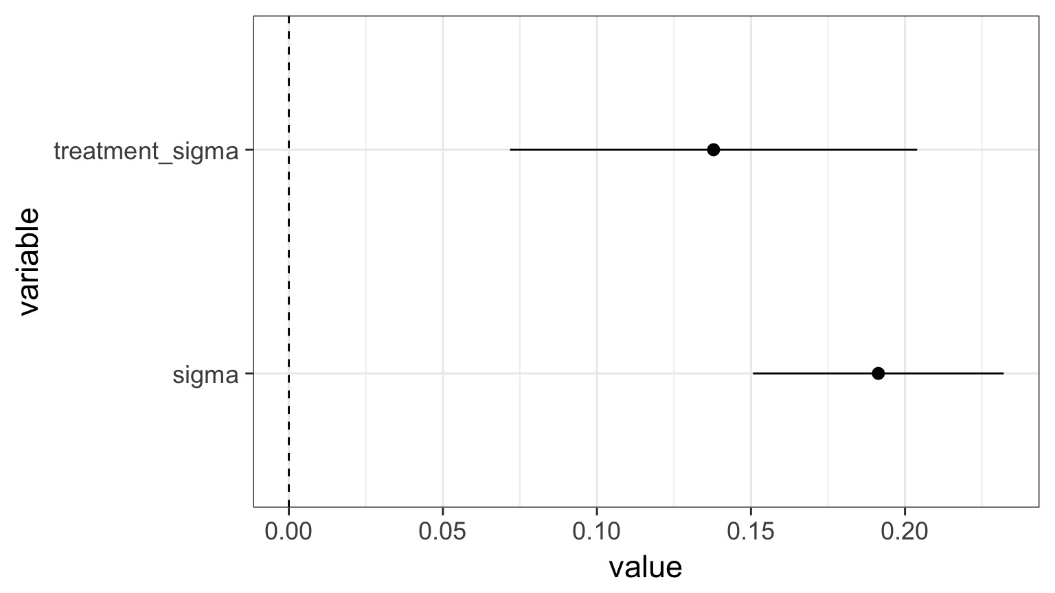
sigma          0.19   0.02  0.16  0.17  0.19  0.22  0.23
mean_PPD      -0.15   0.04 -0.22 -0.20 -0.15 -0.10 -0.09
log-posterior  4.22   1.37  1.57  2.40  4.55  5.65  5.81

Diagnostics:
              mcse Rhat n_eff
groupcontrol  0.00 1.00 3252 
groupschizo   0.00 1.00 3444 
groupbipolar  0.00 1.00 3646 
sigma         0.00 1.00 3137 
mean_PPD      0.00 1.00 3737 
log-posterior 0.03 1.00 2171 

For each parameter, mcse is Monte Carlo standard error, n_eff is a crude measure of effective sample size, and Rhat is the potential scale reduction factor on split chains (at convergence Rhat=1).

BANOVA

                10%    90%
groupcontrol -0.066  0.058
groupschizo  -0.255 -0.134
groupbipolar -0.322 -0.202
sigma         0.167  0.218

What are the sources of variation from the model?

We can look at the SD between means from a set of categorical predictors
This SD tells us how much variability is driven by a set of treatments
Not directly comparable to MSE for comparison to sigma.
Given units of response variable, is the variability meaningful?

What are the sources of variation from the model?

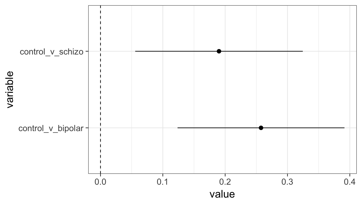
Are Groups Different?

Control v. Schizo

    0%    25%    50%    75%   100% 
-0.054  0.146  0.189  0.234  0.489


Control v. Bipolar

   0%   25%   50%   75%  100% 
0.021 0.214 0.258 0.301 0.531

Alternate methods

Likelihood uses \(\chi^2\), but other methods are identical to least squares
Bayesian methods conservative, but use chains for identical inferences to ANOVA
Sidenote: Bayesian methods are less likely to commit type II errors