Bayesian Statistics: an introduction
Deriving Truth from Data
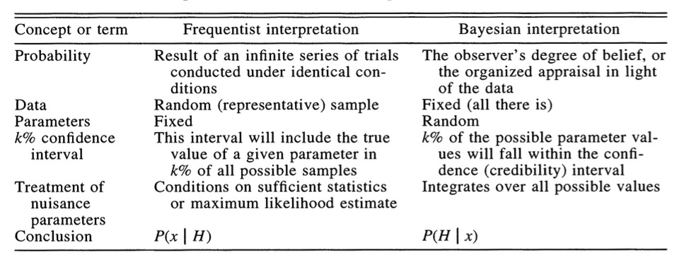
- Frequentist Inference: Correct conclusion drawn from repeated experiments
- Uses p-values and CIs as inferential engine
- Uses p-values and CIs as inferential engine
- Likelihoodist Inference: Evaluate the weight of evidence for different hypotheses
- Derivative of frequentist mode of thinking
- Uses model comparison (sometimes with p-values…)
- Derivative of frequentist mode of thinking
- Bayesian Inference: Probability of belief that is constantly updated
- Uses explicit statements of probability and degree of belief for inferences
Similarities in Frequentist and Likelihoodist Inference
Frequentist inference with Linear Models
Estimate ’true’ slope and intercept
State confidence in our estimate
Evaluate probabilty of obtaining data or more extreme data given a hypothesis
Likelihood inference with Linear Models
Estimate ’true’ slope and intercept
State confidence in our estimate
Evaluate likelihood of data versus likelihood of alternate hypothesis
Bayesian Inference
Estimate probability of a parameter
State degree of believe in specific parameter values
Evaluate probability of hypothesis given the data
Incorporate prior knowledge
- Frequentist: p(x ≤ D | H)
- Likelhoodist: p( D | H)
- p(H | D)
Why is p(H | D) awesome?
- Up until now we have never thought about the probability of a hypothesis
- The probability data (or more extreme data) given a hypothesis provides an answer about a single point hypothesis
- We have been unable to talk about the probability of different hypotheses (or parameter values) relative to one another
- p(H | D) results naturally from Bayes Theorey
Bayes Theorem
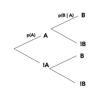
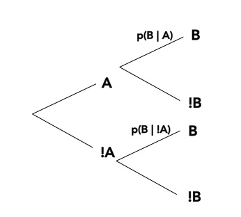
We know…\[\huge p(a\ and\ b) = p(a)p(b|a)\]
Bayes Theorem
And Also…\[\huge p(a\ and\ b) = p(b)p(a|b)\]
Bayes Theorem
And so…
\[\huge p(a)p(b|a) = p(b)p(a|b) \]
Bayes Theorem
And thus…
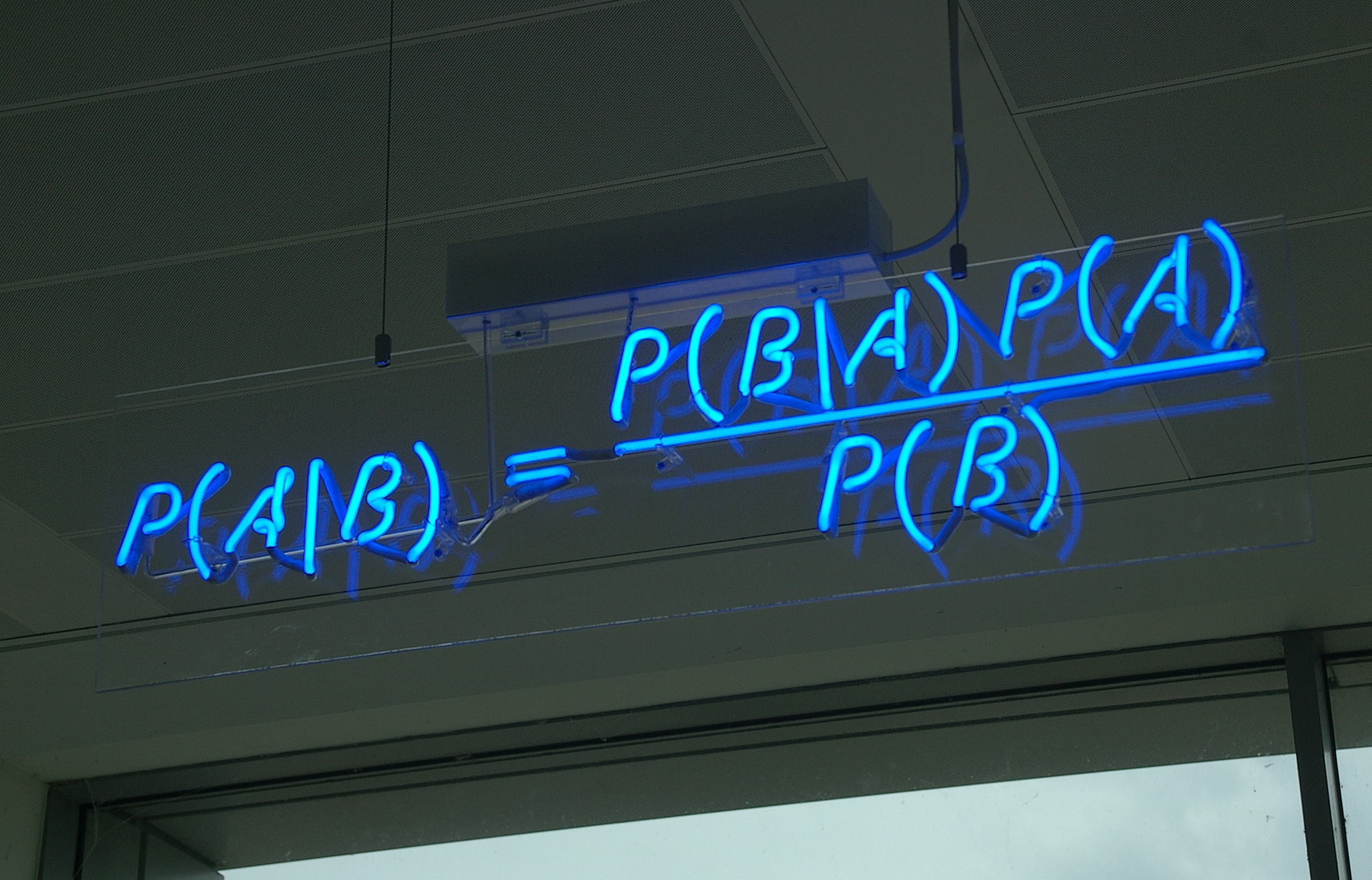
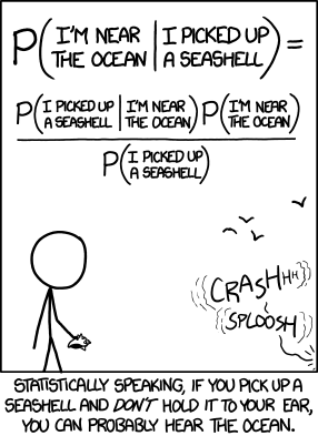
\[\huge p(a|b) = \frac{p(b|a)p(a)}{p(b)} \]

Bayes Theorem and Data
\[\huge p(H|D) = \frac{p(D|H)p(H)}{p(D)} \]
where p(H|D) is your posterior probability of a hypothesis
What is a posterior distribution?
What is a posterior distribution?
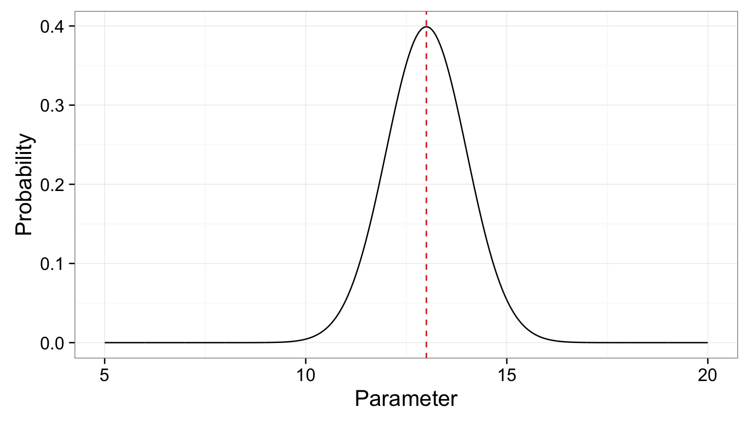
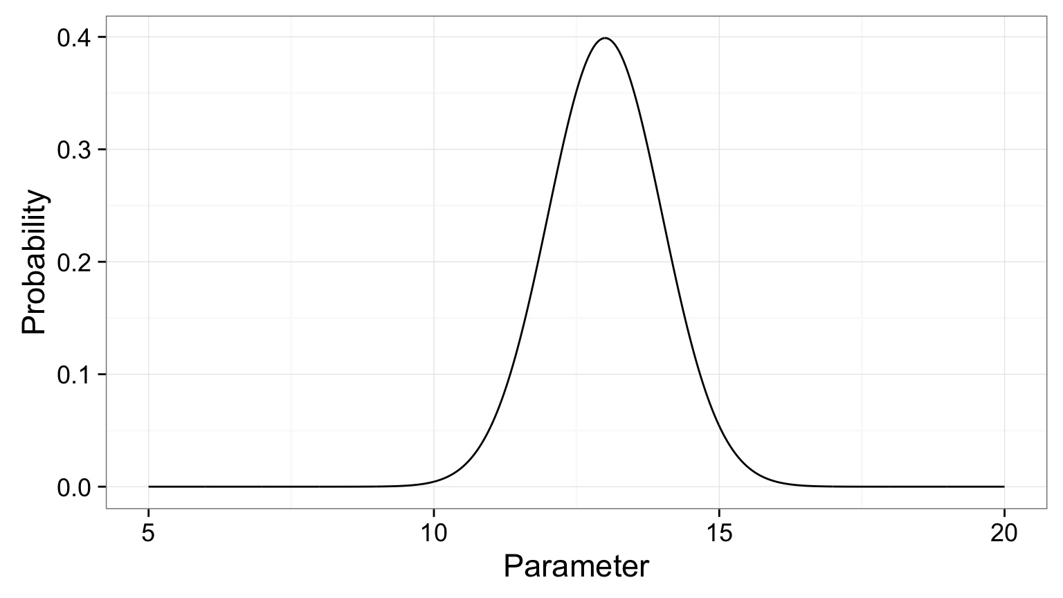
The probability that the parameter is 13 is 0.4
What is a posterior distribution?
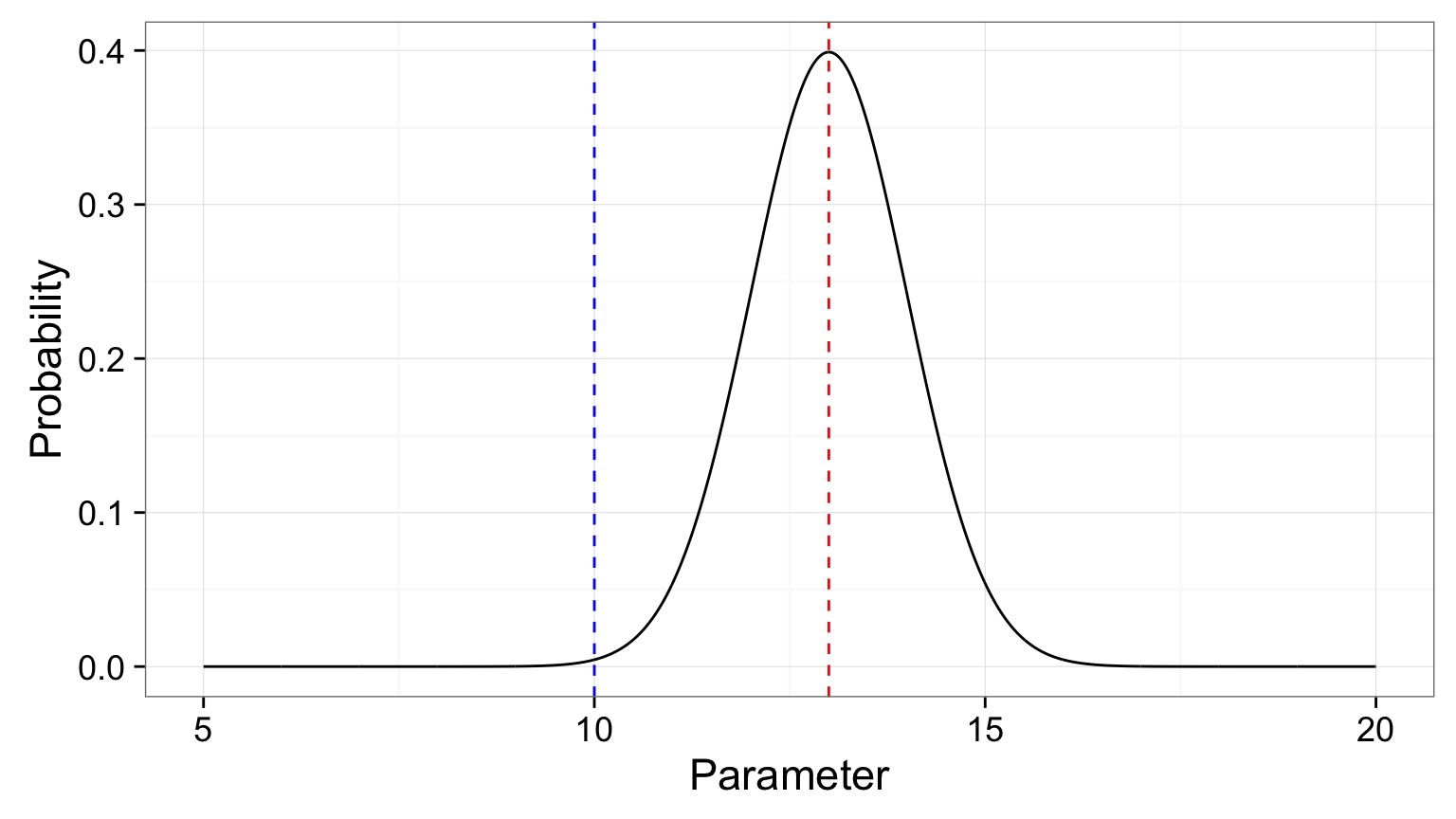
The probability that the parameter is 13 is 0.4 The probability that the parameter is 10 is 0.044
What is a posterior distribution?
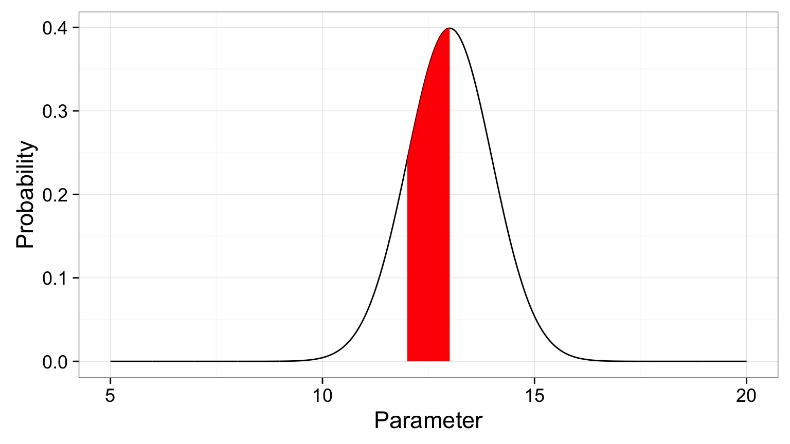
Probability that parameter is between 12 and 13 = 0.3445473
Bayesian Credible Interval
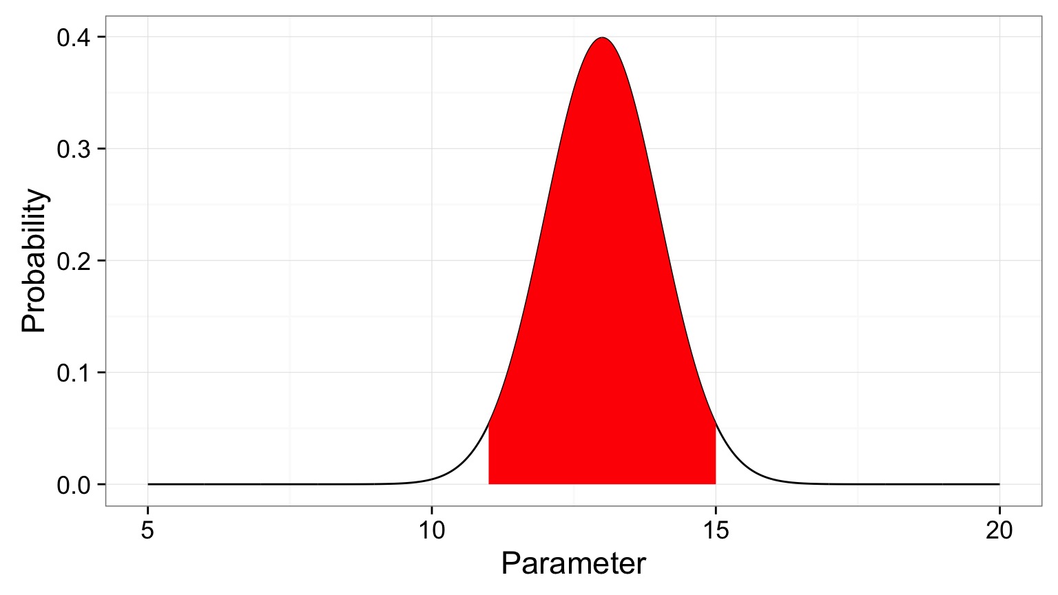
Area that contains 95% of the probability mass of the posterior distribution
Evaluation of a Posterior: Bayesian Credible Intervals
In Bayesian analyses, the 95% Credible Interval is the region in which we find 95% of the possible parameter values. The observed parameter is drawn from this distribution. For normally distributed parameters:
\[\hat{\beta} - 2*\hat{SD} \le \hat{\beta} \le \hat{\beta} +2*\hat{SD}\]
where \(\hat{SD}\) is the SD of the posterior distribution of the parameter \(\beta\). Note, for non-normal posteriors, the distribution may be different.
Evaluation of a Posterior: Frequentist Confidence Intervals
\[\hat{\beta} - t(\alpha, df)SE_{\beta} \le \beta \le \hat{\beta} +t(\alpha, df)SE_{\beta}\]
Credible Intervals versus Confidence Intervals
- Frequentist Confidence Intervals tell you the region you have confidence a true value of a parameter may occur
- If you have an estimate of 5 with a Frequentist CI of 2, you cannot say how likely it is that the parameter is 3, 4, 5, 6, or 7
- Bayesian Credible Intervals tell you the region that you have some probability of a parameter value
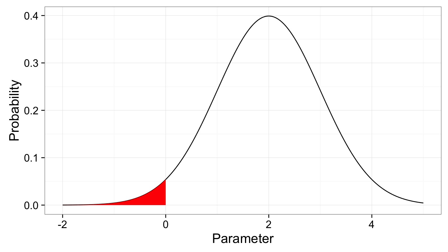
- With an estimate of 5 and a CI of 2, you can make statements about degree of belief in whether a parmeter is 3, 4,5, 6 or 7 - or even the probability that it falls outside of those bounds
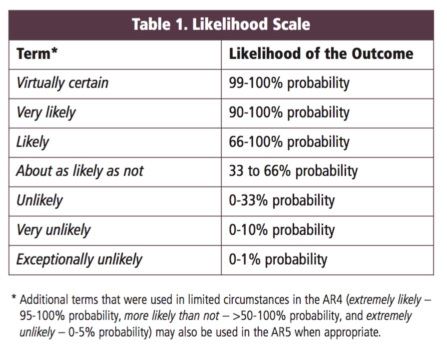
Degree of believe in a result
Talking about Uncertainty the IPCC Way
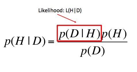
What are the other parts of Bayes Theorem?
\[\huge p(H|D) = \frac{p(D|H)p(H)}{p(D)} \]
where p(H|D) is your posterior probability of a hypothesis
Hello Again, Likelihood
Prior Probability
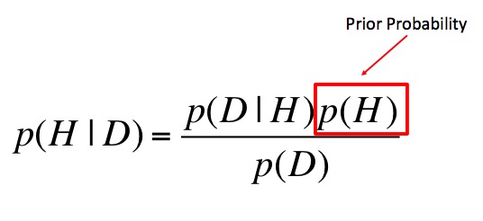
This is why Bayes is different from Likelihood!</span
How do we Choose a Prior?
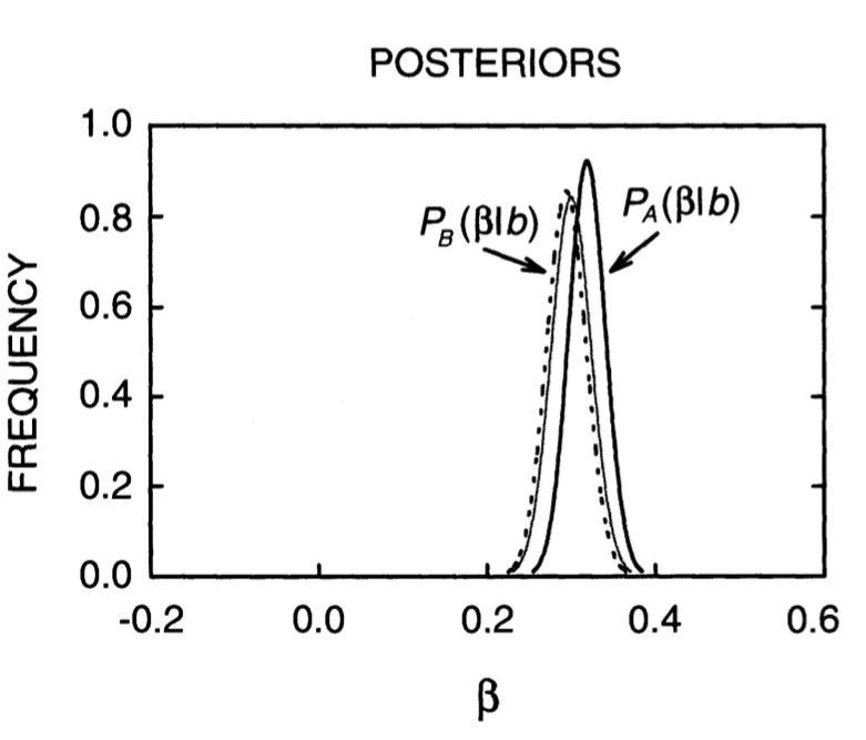
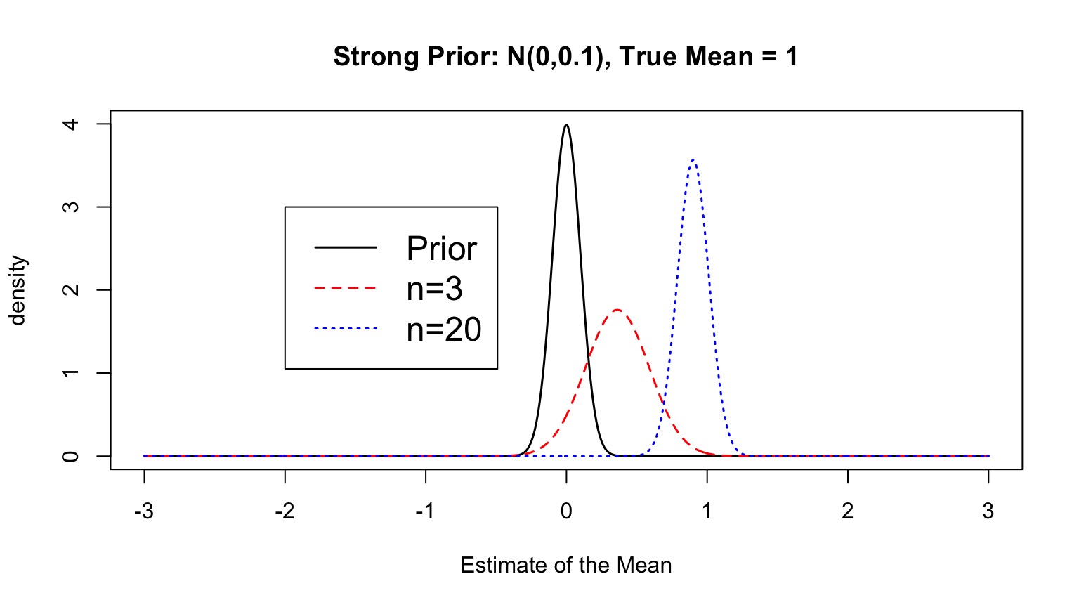
- A prior is a powerful tool, but it can also influence our results of chosen poorly. This is a highly debated topic.
- Conjugate priors make some forms of Bayes Theorem analytically solveable
- If we have objective prior information - from pilot studies or the literature - we can use it to obtain a more informative posterior distribution
- If we do not, we can use a weak or flat prior (e.g., N(0,1000)). Note: constraining the range of possible values can still be weakly informative - and in some cases beneficial
The Influence of Priors
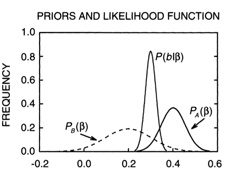
The Influence of Priors
Priors and Sample Size
p(data) is just a big summation/integral
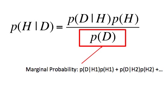

Denominator: The Marginal Distribution

Essentially, all alternate hypotheses
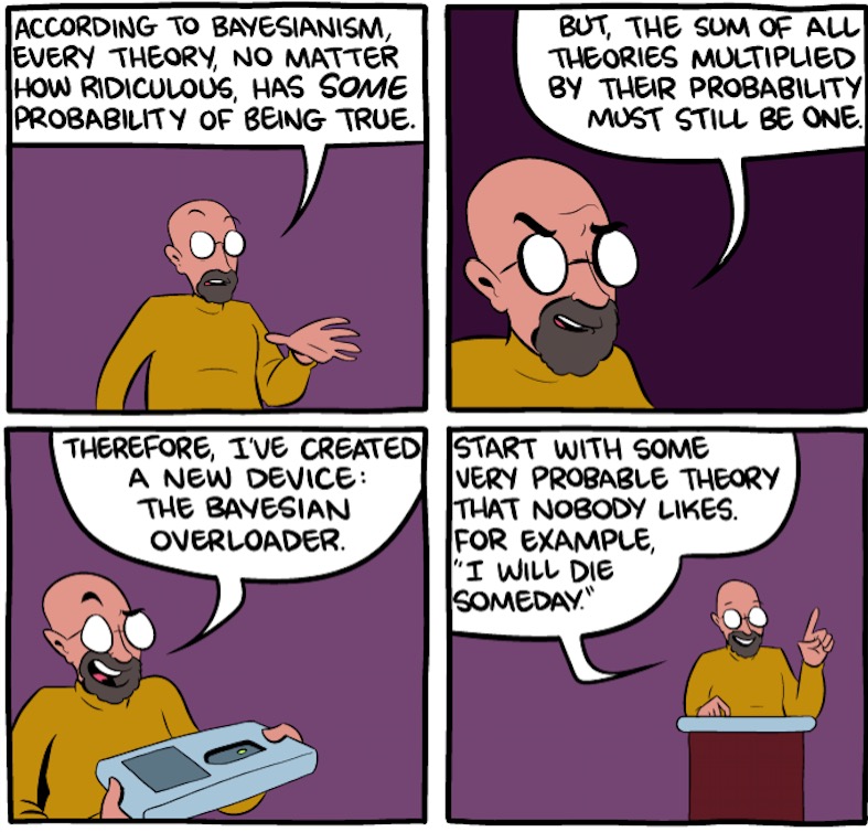
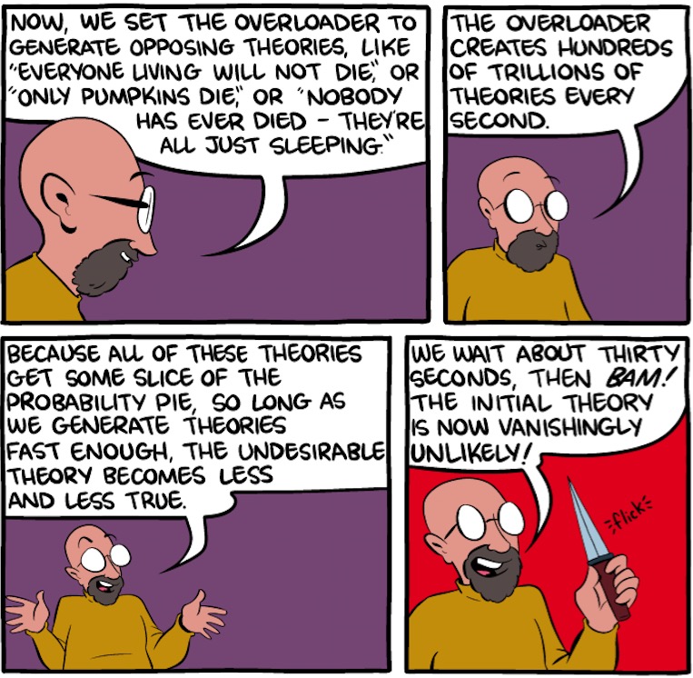
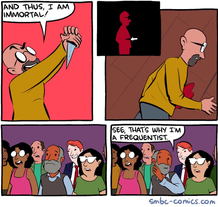
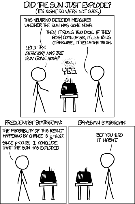
Bayes Theorem in Action

Bayes Theorem in Action
\[p(Sun Explodes | Yes) = \frac{p(Yes | Sun Explodes)p(Sun Explodes)}{p(Yes)}\]
We know/assume:
p(Sun Explodes) = 0.0001, P(Yes \(|\) Sun Explodes) = 35/36
So…
p(Yes) = P(Yes \(|\) Sun Explodes)p(Sun Explodes)
= 35/36 * 0.0001
= 9.7e10^-5
credit: Amelia Hoover
Bayes Theorem in Action
\[p(Sun Explodes | Yes) = \frac{p(Yes | Sun Explodes)p(Sun Explodes)}{p(Yes)}\]
We can calculate:
p(Yes) = P(Yes \(|\) Sun Explodes)p(Sun Explodes) +
P(Yes \(|\) Sun Doesn’t Explode)p(Sun Doesn’t Explodes)
= 35/36 * 0.0001 + 1/36 * 0.9999
= 0.0277775
credit: Amelia Hoover
Bayes Theorem in Action
\[p(Sun Explodes | Yes) = \frac{p(Yes | Sun Explodes)p(Sun Explodes)}{p(Yes)}\]
\[p(Sun Explodes | Yes) = \frac{0.0001*35/36}{0.028}\] \[= 0.0035\]
Incorporating Prior Information about the Sun Exploding gives us a very different answer
Note, we can also evaluate the probability of the alternate hypothesis - p(Sun Doesn’t Explode \(|\) Yes)
Where have we gone?
